Chapter 2 Dataset

The data is sourced as a SQLite database that downloaded from teh Kaggle website (Preparation: Wendy Kan 2019) and imported as a tibble dataframe with the RSQLite package. The variables were reformatted according to their respective types. The full list of variable is given in Appendix (see Table ??). This dataset will be reduced as we focused on the core intent of modeling the probability of default.

Note that the dataset was anonymised (all identifying ID numbers are deleted) and we therefore removed the corresponding empty columns from the dataset. Since the identification IDs have been removed to anonymise the dataset, we cannot see if a borrower borrowed several times.

2.1 Preamble

The LendingClub dataset, although rich, is difficult to interpret. The only explanation of what the variables mean comes from a spreadsheet attached to the dataset. The explanations are not precise and/or subject to conflicting interpretation. Despite serching the LendingClub website, no further original information was found. We collected a number of reasonable assumptions in Appendix (see subsection 6.1 in Appendix).

The dataset has been used a number of times in the past by various people. One paper (Kim and Cho 2019) mentions they used a dataset that included 110 variables, which is less than ours with 145 variables. It is therefore clear that the dataset has changed over time in ways we do not know. For example, have loans been excluded because the full 145 veriables were not available?

2.2 General presentation

The original dataset is large: it includes 2260668 loan samples, each containing 145 variables (after the identification variables filled with null values). The loans were issued from 2007-06-01 to 2018-12-01.

2.2.1 Business volume

The dataset represents a total of ca.$34bln in loan principals, which is a substantial share of the total amount stated to have been intermediated to date by LC (publicly reported to be $50bln+). About 55%/60% of the portfolio is not current anymore (either fully or partially repaid). See Table ??.

Figure 2.1 plots the number, volume (cumulative principal amount) and average principal per loan. It shows that the business grew exponentially (in the common sense of the word) from inception until 2016. At this point, according to Wikipedia:⁷

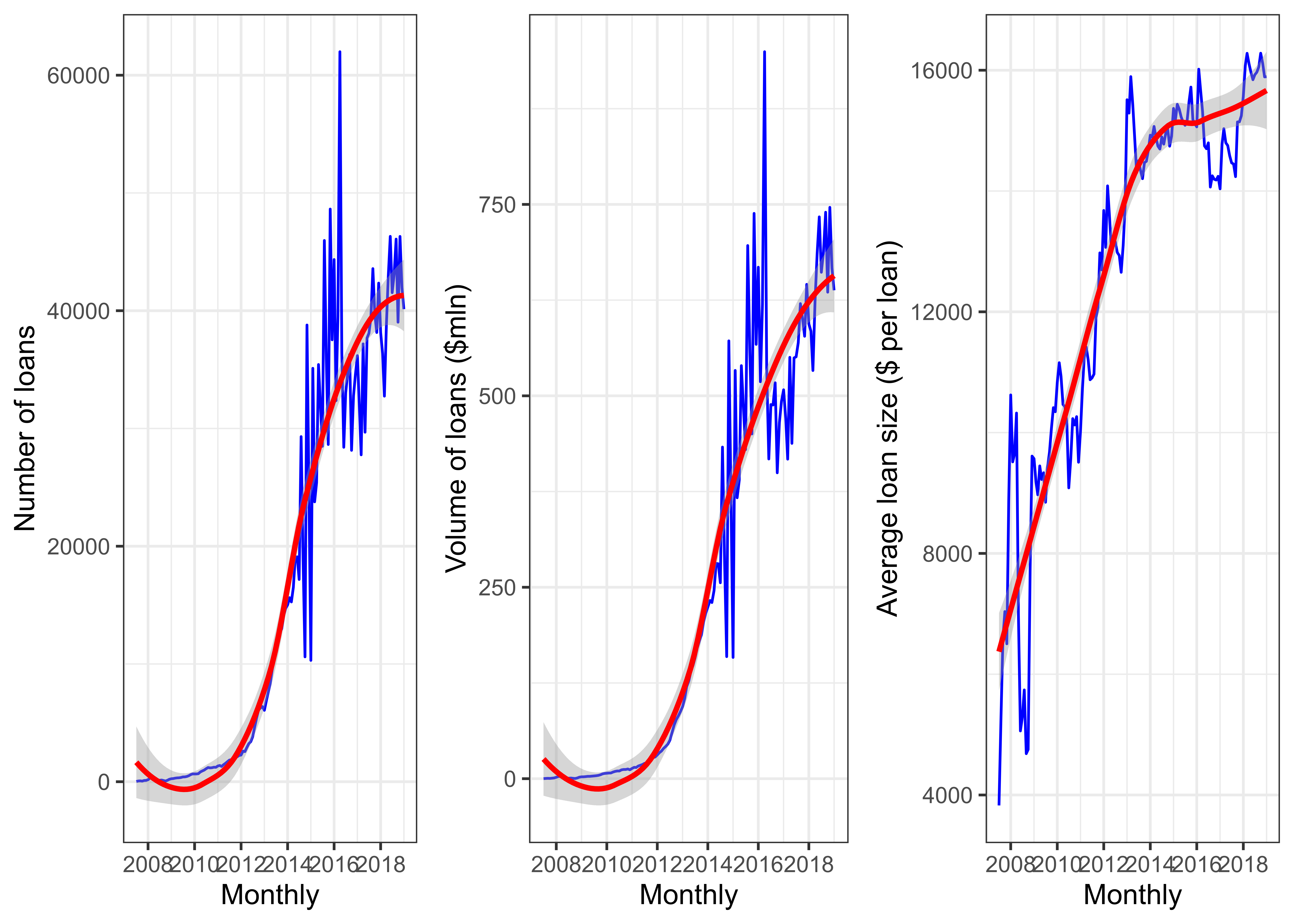
Figure 2.1: Business volume written per month

" Like other peer-to-peer lenders including Prosper, Sofi and Khutzpa.com, LendingClub experienced increasing difficulty attracting investors during early 2016. This led the firm to increase the interest rate it charges borrowers on three occasions during the first months of the year. The increase in interest rates and concerns over the impact of the slowing United States economy caused a large drop in LendingClub’s share price."

The number and volume of loans plotted have been aggregated by month. The growth is very smooth in the early years, and suddenly very volatile. As far as the first part of the dataset is concerned, a starting business could expect to be volatile and could witness a yearly cycle (expected from economic consumption figures) superimposed on the growth trend. This is not the case.

An interesting metric is that the average principal of loans has increased (see RHS Figure 2.1, on a sample of 100,000 loans). Partly, the increase in the early years could be interpreted success in improving marketing, distribution capabilities and confidence building. This metric plateau-ed in 2016 and decreased afterwards, but to a much lesser extent than the gross volume metrics. However, it is more volatile than the two previous metrics in the early years.

By the end of the dataset, those metrics have essentially recovered to their 2016 level.

2.2.2 Loan lifecyle and status

In the dataset, less loans are still outstanding than matured or “charged off” (term that LC use to mean partially or fully written off, i.e. there are no possibilty for LC and/or the investors to receive further payments). The share of outstanding loans is:

## Share of current loans =  42.214 %

The dataset describes the life cycle of a loan. In the typical (ideal) case, we understand it to be:

\[ \text{Loan is approved} \rightarrow \text{Full amount funded by investors} \rightarrow \text{Loan marked as Current} \rightarrow \text{Fully Paid} \]

In the worst case, it is:

\[ \text{Loan is approved} \rightarrow \text{Full amount funded by investors} \rightarrow \text{Loan marked as Current} \rightarrow \]

\[ \rightarrow \text{Grace period (missed payments under 2 weeks)} \rightarrow \text{Late 15 to 31 days} \rightarrow \]

\[ \rightarrow \text{Late 31 to 120 days} \rightarrow \text{Default} \rightarrow \text{Charged Off} \]

Note that Default precedes and is distinct from Charged Off.⁸ A couple of things could happen to a loan in default:

• LC and the borrower restructure the loan with a new repayment schedule, where the borrower may repay a lesser amount over a longer period; or,

• the claim could be sold to a debt recovery company that would buy the claim from LC/investors. This would be the final payment (if any) received by LC and the investors.

The dataset also describes situations where a borrower negotiated a restructuring of the repayment schedule in case of unexpected hardship (e.g. disaster, sudden unemployment).

Note that this progression of distinguishing default (event in time) from actual financial loss mirrors what banks and rating agencies do. The former is called the Probability of Default (PD), the latter Loss Given Default (LGD). Ratings change over time (in a process resembling Markov Chains transitions). LGD show some correlations with ratings. The dataset, although detailed, does not include the full life of each loan to conduct this sort of analysis (change of loan quality over time). This is an important reason why we decided to focus on the loan approval and expected return.

2.2.3 Loan application

Before a loan is approved, the borrower undergoes a review process that assess his/her capacity to repay. This includes:

• employment situation and income, as well whether this income and possibly its source has been independently verified;

• whether the application is made jointly (likely with a partner or a spouse, but there are no details);

• housing situation (owner, owner with current mortgage, rental) and in which county he/she lives (that piece of information is partially anonymised by removing the last 2 digits of the borrower’s zipcode);

• the amount sought, its tenor and the purpose of the loan; and,

• what seems to be previous credit history (number of previous deliquencies). The dataset is very confusing in that regard: in the case of the joint applicant, it is clear that such information relates to before the loan is approved . In the case of the principal borrower however, the variable descriptions could be read as being pre-approval information, or post-approval gathered during the life of the loan. We have assumed that the information related to the principal borrower is also pre-approval. We also used Sales Supplements from the LC website⁹ that describe some of the information provided to investors. LendingClub also provides a summary description of its approval process in its regulatory filings with the Securities Exchange Commission (San Francisco - California 2019).

2.3 Rates

2.3.1 IRR and required credit margins

Figure 2.2 shows the evolution of credit margins over time grouped by ratings. The plots are made with a random sample of 300,000 loans.

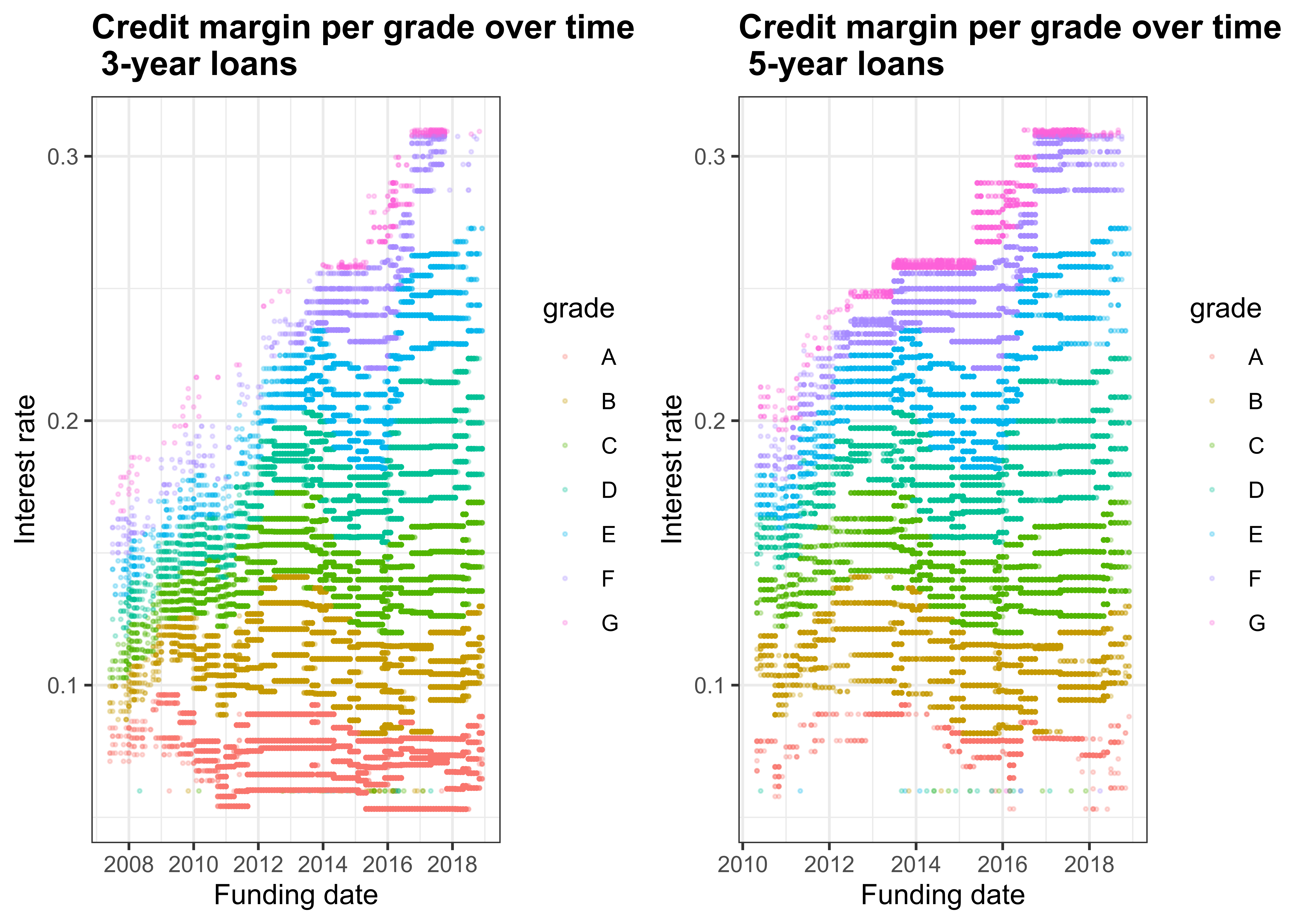
Figure 2.2: Credit margins per grade over time

We notice long periods where certain margins remain fairly stable which indicate that both the initial pricing was constant and that the proportion of default remains very low.

The graphs offer considerations that are relevant to the modeling:

• The margins clearly change over time. To the extent that they reflect a change in probability of default, the predictions will require to account for time (probably in a non-linear fashion).¹⁰

• For a given rating, the margins widen and narrow over time. The changes happen in multiples that depends on the ratings:

  • For high quality / low margin loans: the changes are multiples of the margin, for example going from roughly 3% to 6/7%.

  • Although the range of change is wide, those changes do not happen very often, especially in the later years.

  • By comparison, for low quality / high margin loans, the range of change is proportionally smaller, but more frequent and volatile.

• In other words, the relation between loan quality (its rating) and its pricing (the credit margin) will significantly non-linear.

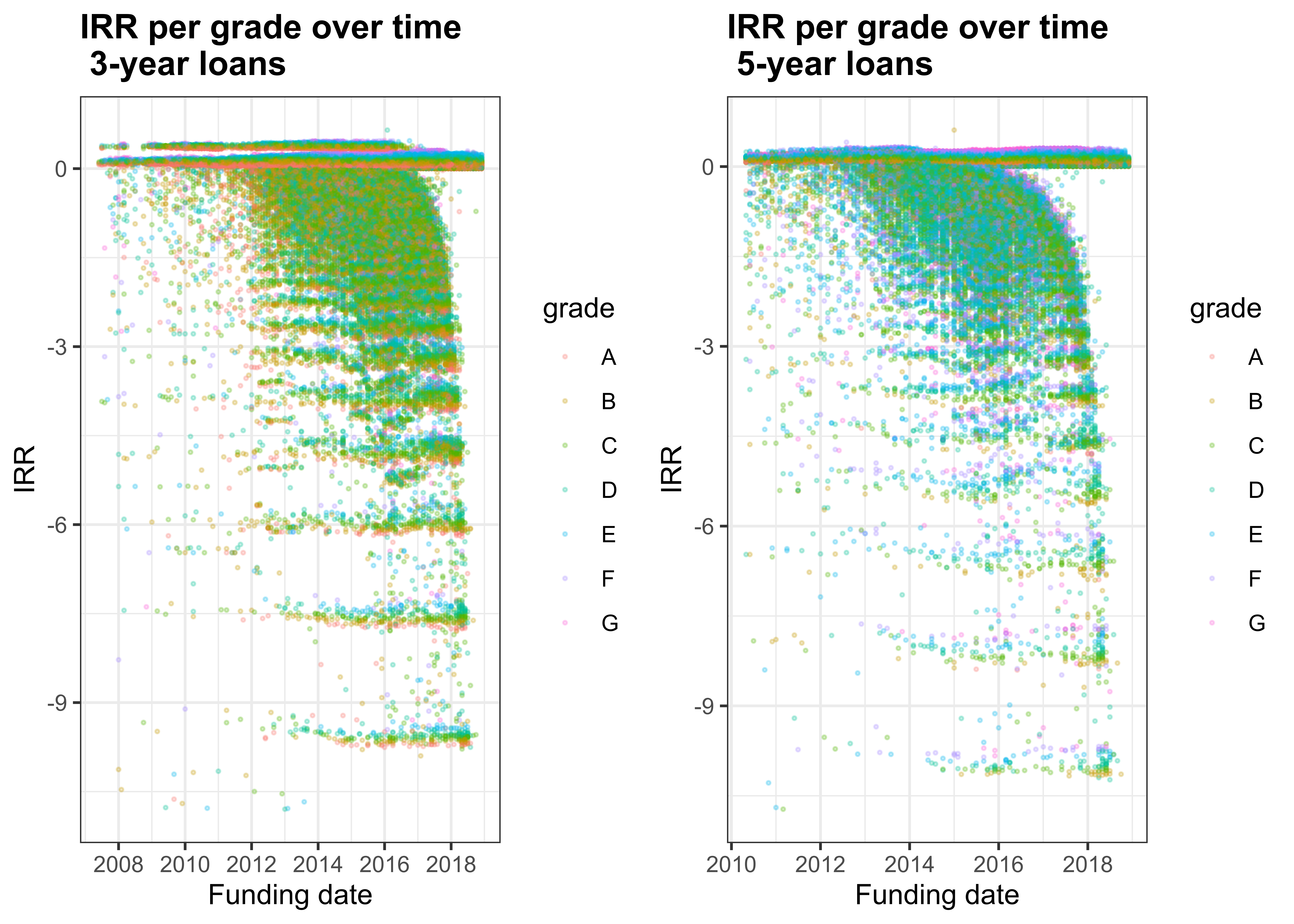
Figure 2.3: Credit margins per grade over time

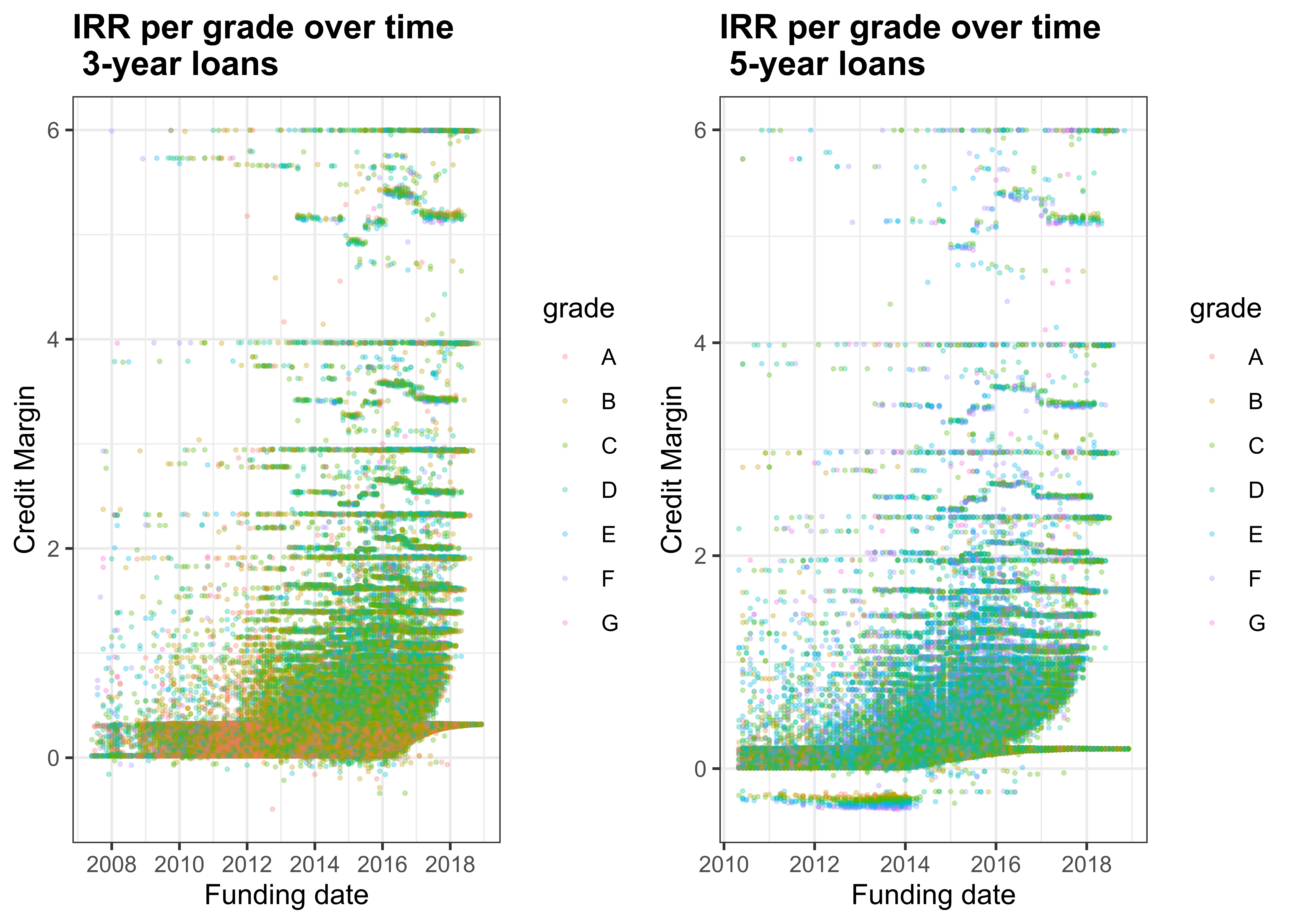
Figure 2.4: Credit margins per grade over time

2.3.2 Choice of predictors

Because we are interested decisions made prior to invest, we will limit the predictors to those that are realistically available prior to funding. We also remove information that is provided as a result of LC’s own credit analysis (e.g. grade and interest rate).

2.3.3 Interest rates

Based on this information, the loan is approved or not. Approval includes the final amount (which could be lower than the amount requested), tenor (3 or 5 years) and a rating similar to those given to corporate borrowers. Unlike corporate borrowers however, the rating mechanically determines the rate of interest according to a grid known to the borrower in advance¹¹. The rates have changed over time. Those changes where not as frequent as market conditions (e.g. changes in Federal Reserve Bank’s rates)¹².

Figure 2.5¹³ shows the predetermined interest rate depending on the initial rating as of July 2019.

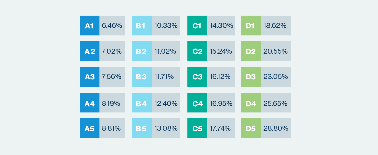
Figure 2.5: Interest rates given rating

At the date of this report, the ratings range from A (the best) down to D, each split in 5 sub-ratings. In the past, LC has also intermediated loans rated F or G (until 6 November 2017) and E (until 30 June 2019).¹⁴ This explains that such ratings are in the dataset. We will assume that the ratings in the dataset are the rating at the time of approval and that, even if loans are re-rated by LC, the dataset does not reflect it.

Figures 2.6 shows the change in interest rate over time for different ratings and separated for each tenor. (Each figure is on a sample of 100,000 loans.) For each rating, we can see several parallel lines which correspond to the 5 sub-rating of each rating. We note that the range of interest rates has substantial widened over time. That is, the risk premium necessary to attract potential investors has had to substantially increase. In the most recent years, the highest rates exceed 30% which is higher than many credit cards.3-year loans are naturally considered safer (more A-rated, less G-rated). Identical ratings attract identical rates of interest.

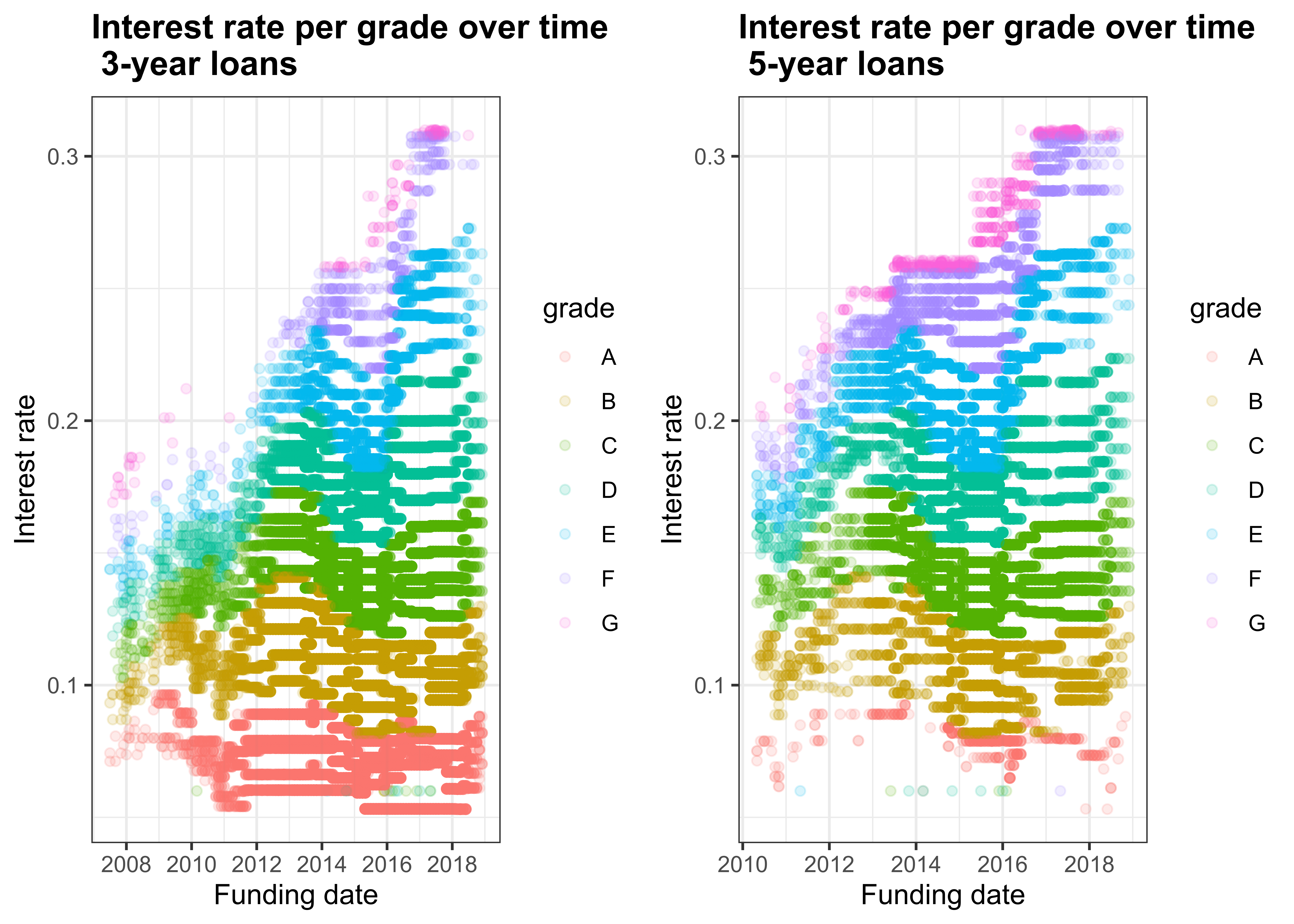
Figure 2.6: Interest rate per grade over time

By comparison, we plot the 3-year (in red) and 5-year (in blue) bank swap rates in Figure 2.7. We see that the swap curve has flattened in recent times (3-year and 5-y rates are almost identical). We also can see that in broad terms the interest rates charged reflect those underlying swap rates. It is more relevant to examine the credit margins excluding swap rates.

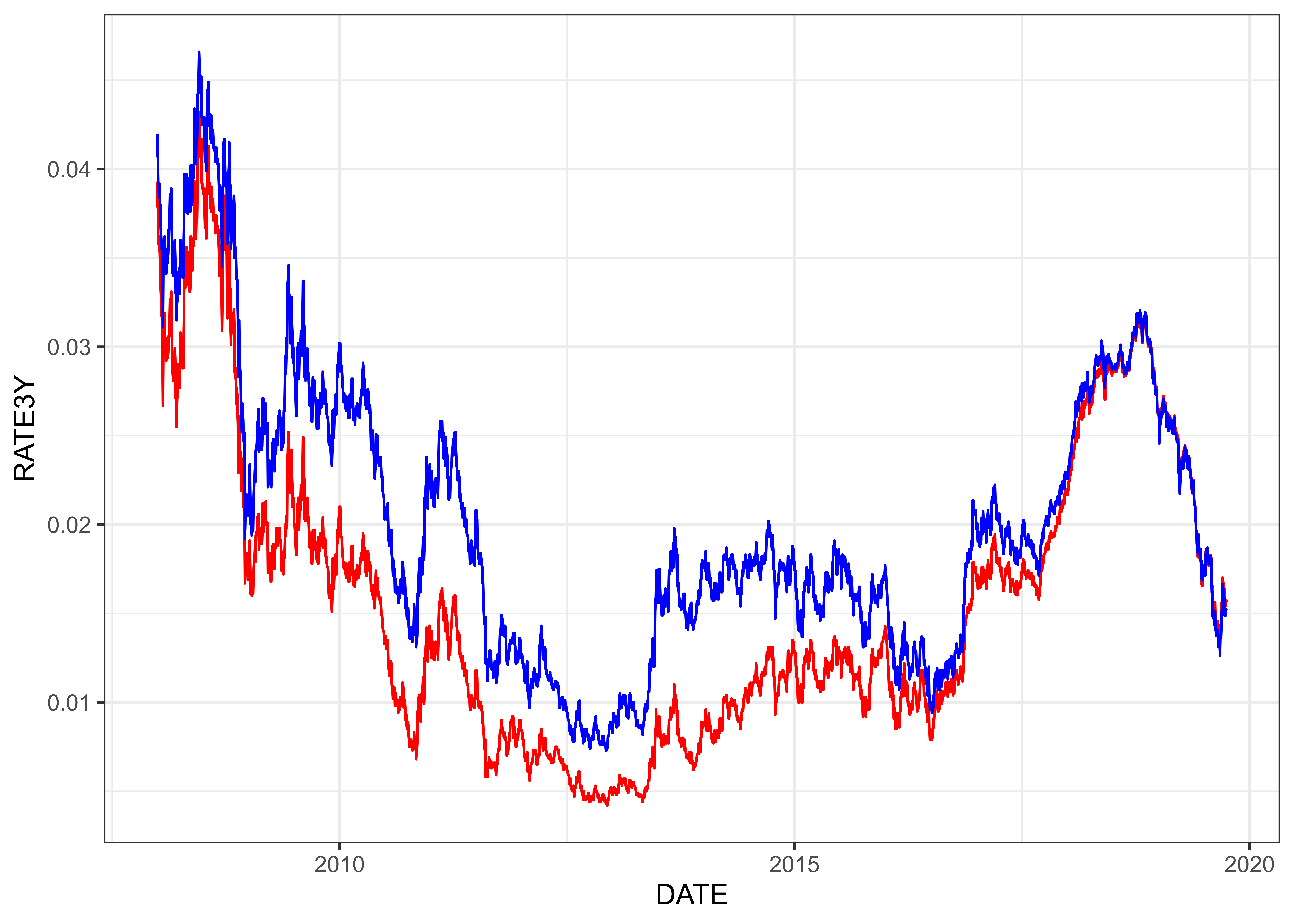
Figure 2.7: Historical Swap Rates

Figures 2.8 shows the change in credit margin over time for different ratings and separated for each tenor. (Each figure is on a sample of 100,000 loans.) As above, for each rating, we can see several parallel lines which correspond to the 5 sub-rating of each rating. We note that the range of credit margins has widened over time but less than the interest rates. Identical ratings attract identical credit margins.

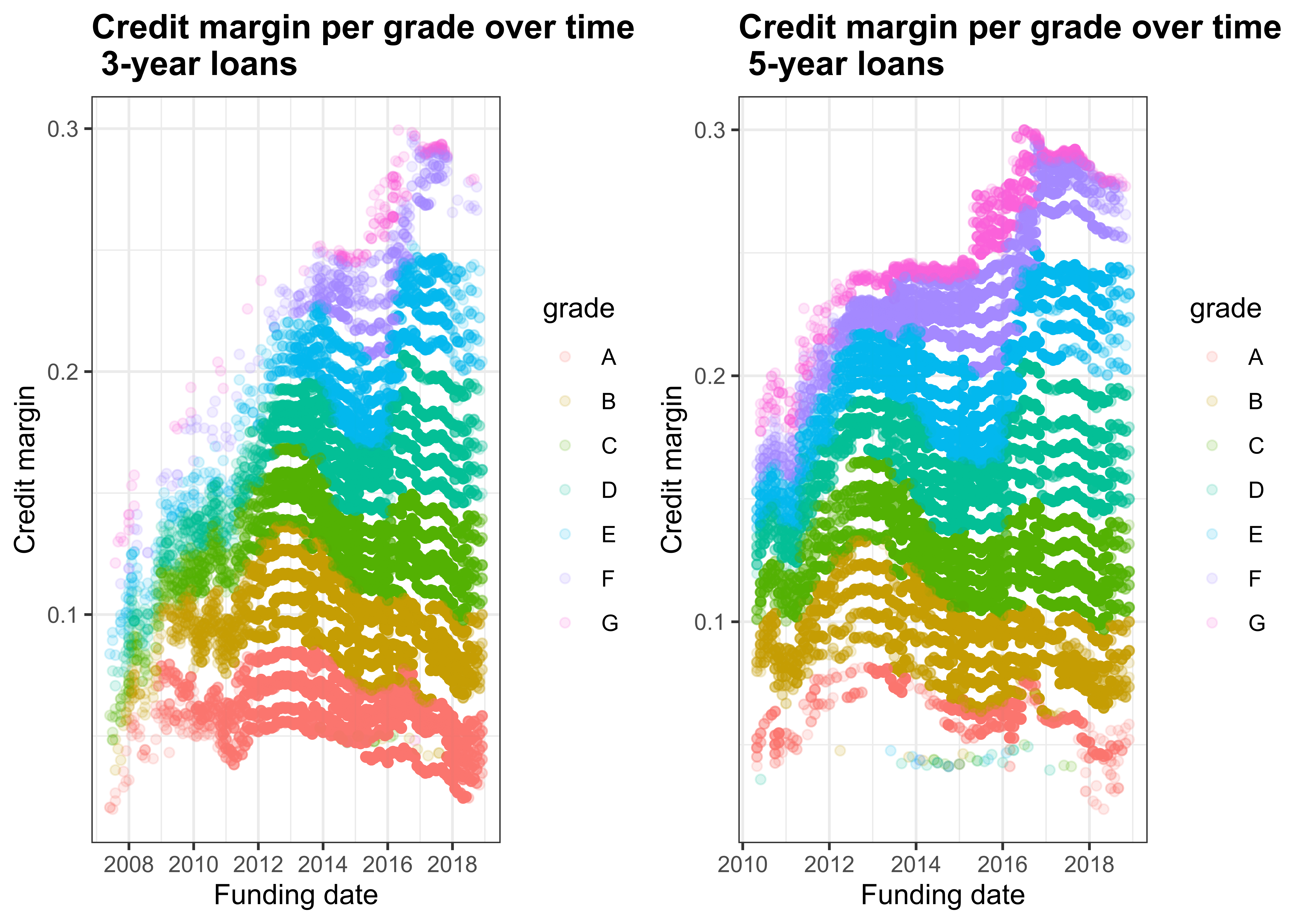
Figure 2.8: Credit margins per grade over time

2.3.4 Purpose

When applying, a potential borrower must state the purpose of the loan. As shown in table ??, by far the main purpose is the consolidation of existing debts.

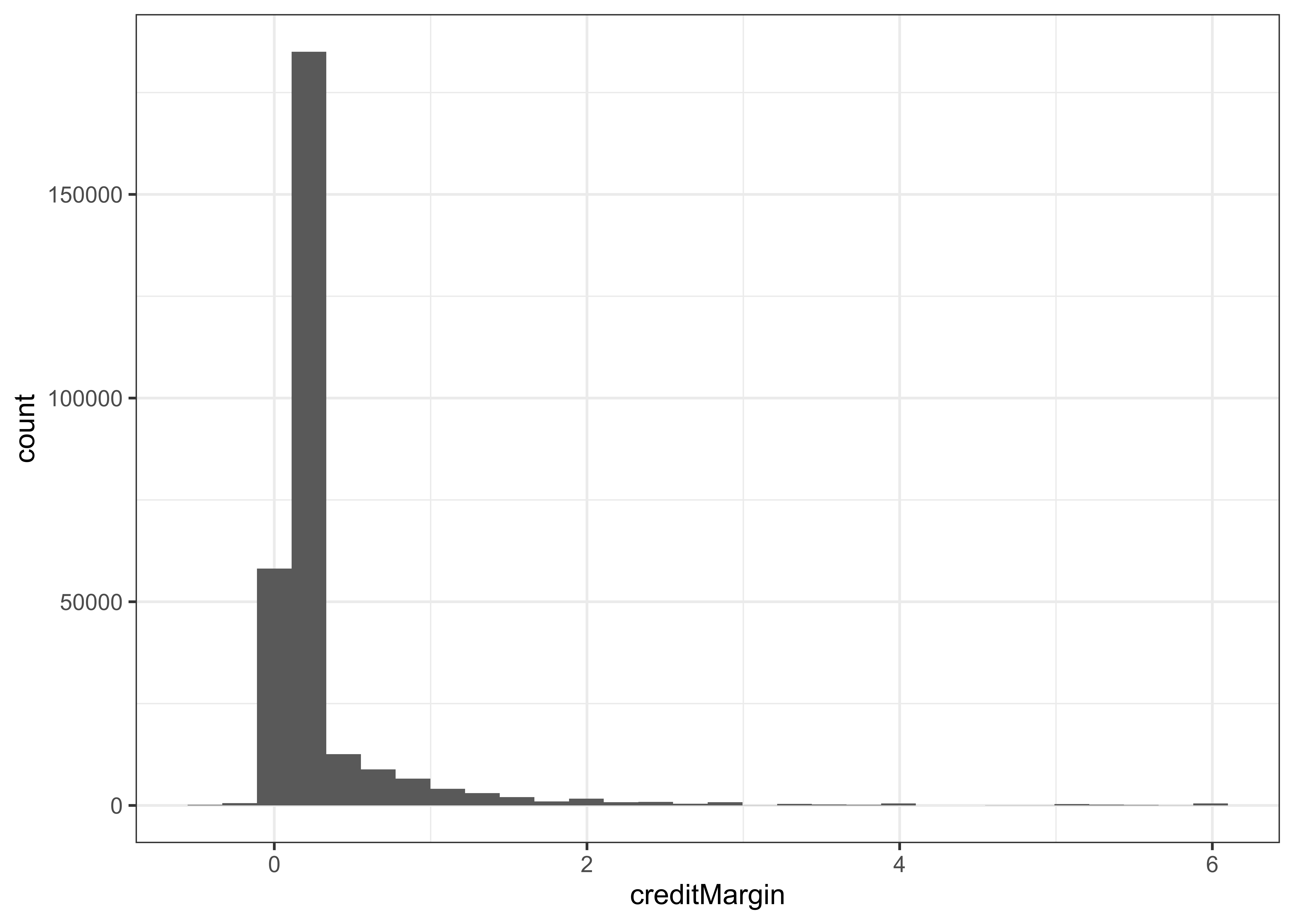
Figure 2.9: Histograms of credit margins per purpose

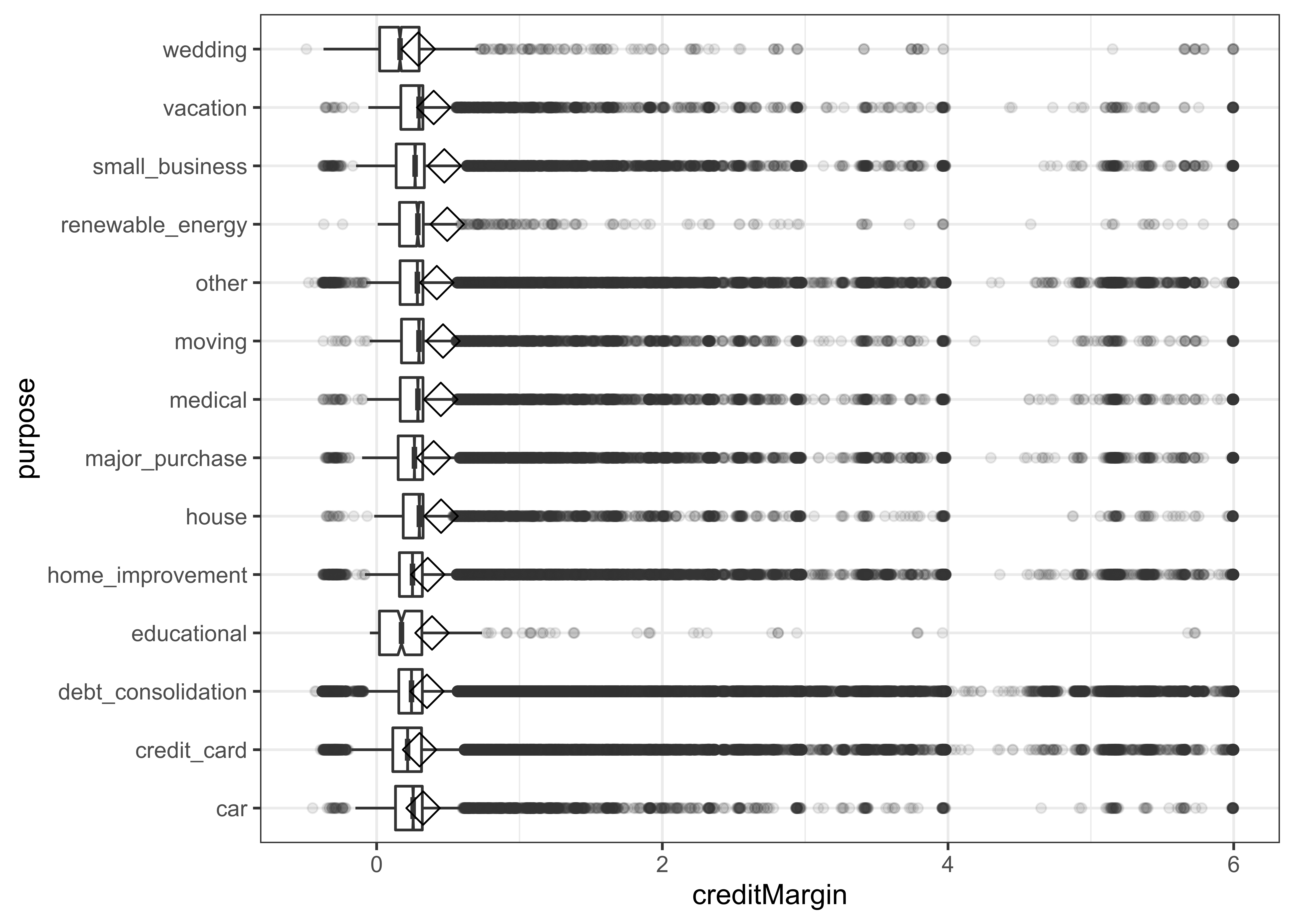
Figure 2.10: Boxplots of credit margins per purpose

2.3.5 Payments

The loans are approved for only two tenors, 3 and 5 years, with monthly repayments. Installments are calculated easily with the standard formula:

\[ Installment = Principal \times rate \times \frac{1}{1 - \frac{1}{(1+rate)^N}} \]

Where \(Principal\) is the amount borrowed, \(rate = \frac{\text{Quoted Interest Rate}}{12}\) is the monthly interest rate, and \(N\) is the number of installments (36 or 60 monthly payments). The following piece of code shows that the average error between this formula and the dataset value is about 2 cents. We therefore precisely understand this variable.

local({
  installmentError <- loans %>%
    mutate(
      PMT = round(funded_amnt * int_rate / 12 / (1 - 1 / (1 + int_rate / 12) ^
                                                   term), 2),
      PMT_delta = abs(installment - PMT)
    ) %>%
    select(PMT_delta)
  
  round(mean(100 * installmentError$PMT_delta), digits = 2)
})

2.4 Net present value

The behaviour of the NPV of loan losses is informative.

2.4.1 Average NPV and credit margin by subgrade

Figure 2.11 shows that as ratings worsen, the average NPV¹⁵ expressed as a portion of the funded amount decreases. For the best quality loans, we see that the NPV exceeds 1.00 = 100%: at a risk-free rate¹⁶, investors receive more than what is necessary to compensate for credit loss and can use the excess to cover additional costs mentioned in the Preamble. As ratings worsen, the NPV drops down to about 50%.

If loans were adequately priced, the excess returns (thanks to higher interest) should on average offset credit losses, that is an NPV average should be at least 100%. This seems to be the case down to ratings of about D4. Further down, credit losses become too frequent and/or too substantial to be covered on average. We posit that this justified rejecting loans applications rated E1 and below.

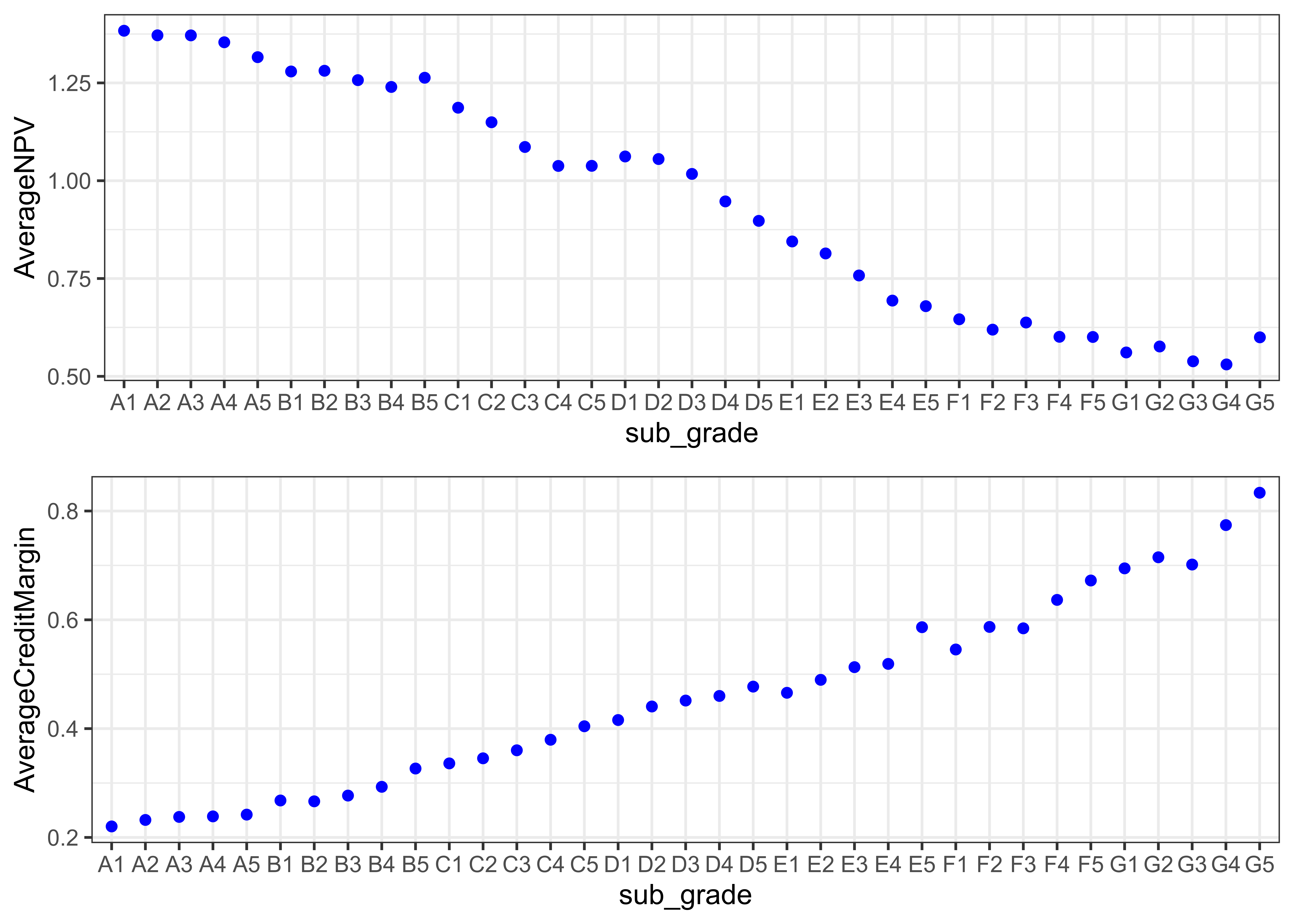
Figure 2.11: Average NPV et credit margin (%) depending on sub-rating

2.4.2 Distribution of principal losses by rating

We here consider nominal losses, that is not accounting for time effects (discounting).

Figure 2.12 shows that for a given grade, the losses are very widely spread. The loans are grouped by ratings and loans that have been fully repaid are removed.

Setting aside the loans rated “A” or “B”, the distributions seem log-normal. Unsurprisingly, the worse the rating the larger the principal loss.

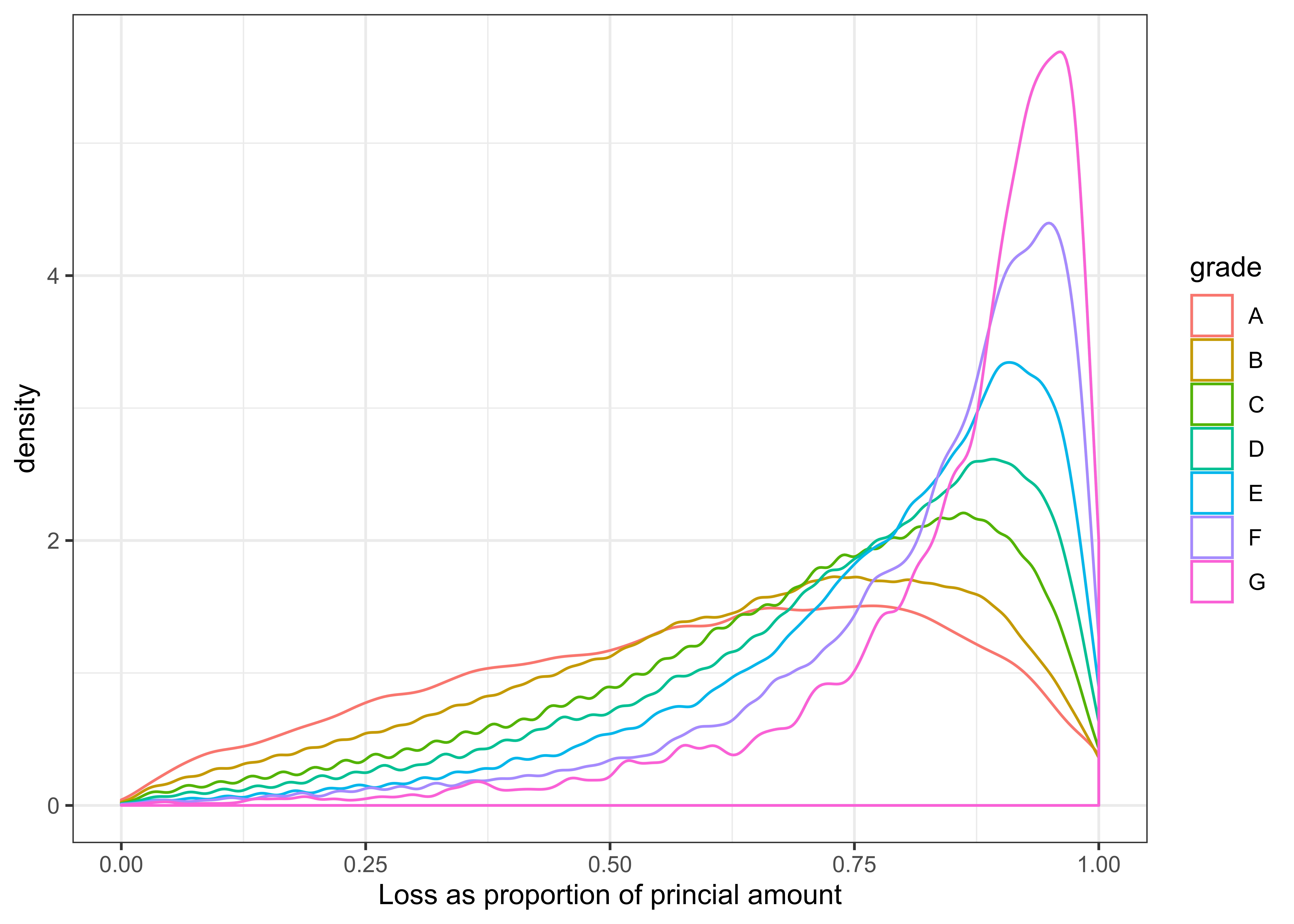
Figure 2.12: Distribution of the Principal Loss (%) depending on rating (y-axis square-root scaling)

2.4.3 NPV distribution by rating

Principal loss does not reflect the timing of that loss: for the same dollar amount, a loss now is worse than a loss later. This subsection looks at the NPVs of actual loan cashflow (principal and interest) discounted the risk-free rate.

Figure 2.13 shows that for a given grade, the NPVs are very widely spread. From top to bottom, loans are group by ratings: from quality ratings of A and B, average ratings of C and D, to poor ratings of E and below. From left to right, we focus on different parts of how NPVs are distributed. Note that each graph is based on a random sample of 100,000 loans (about 1/12th of the original set) and therefore the NPV densities are comparable from graph to graph. This spread is expected. The amount of loss for any loan can be anything a single dollar and 100%.

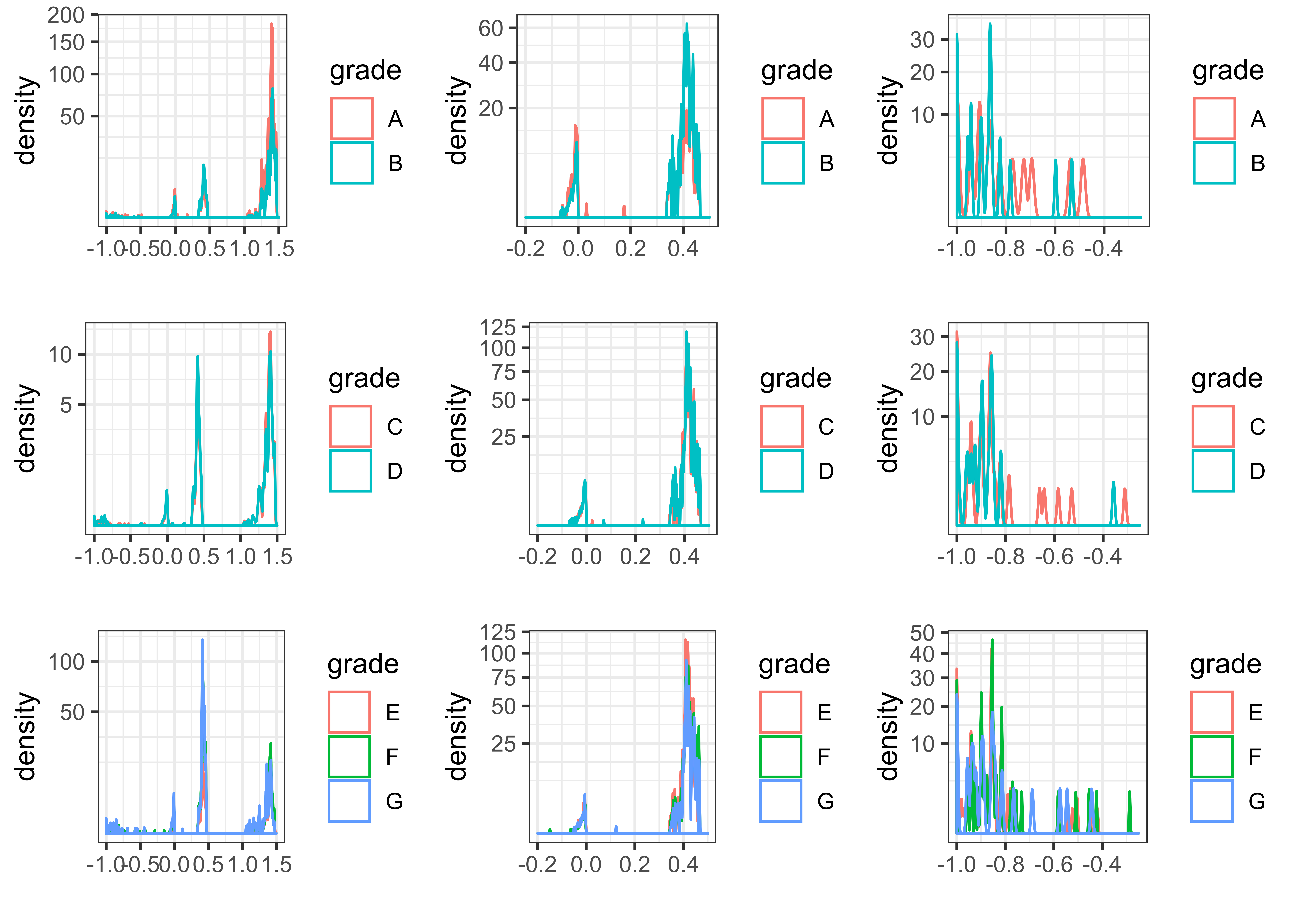
Figure 2.13: Distribution of NPV (%) depending on rating (y-axis square-root scaling)

At the outset, column by column (where NPVs are on the same scale), the NPV distribution show several modes on the same location. The modes are made more apparent by zooming on where the modes are present: the leftmost column basically shows the entire range of the NPVs (as portion of the loan). The middle graph zooms on the -20% / 50% range. The rightmost column zooms on the -100% / -25% section. Looking at the left hand scale, we can see that the lower NPVs overall gain in importance as the loan rating worsen.

Zooming without scaling the y-axis and grouping all the ratings available for investment on a single plot gives more details.

• Figure 2.14 shows a mode with a maximum around 1.25 / 1.5 being loans seemingly repaid in full (the mode is above 100% given the repayment of principal and interest);

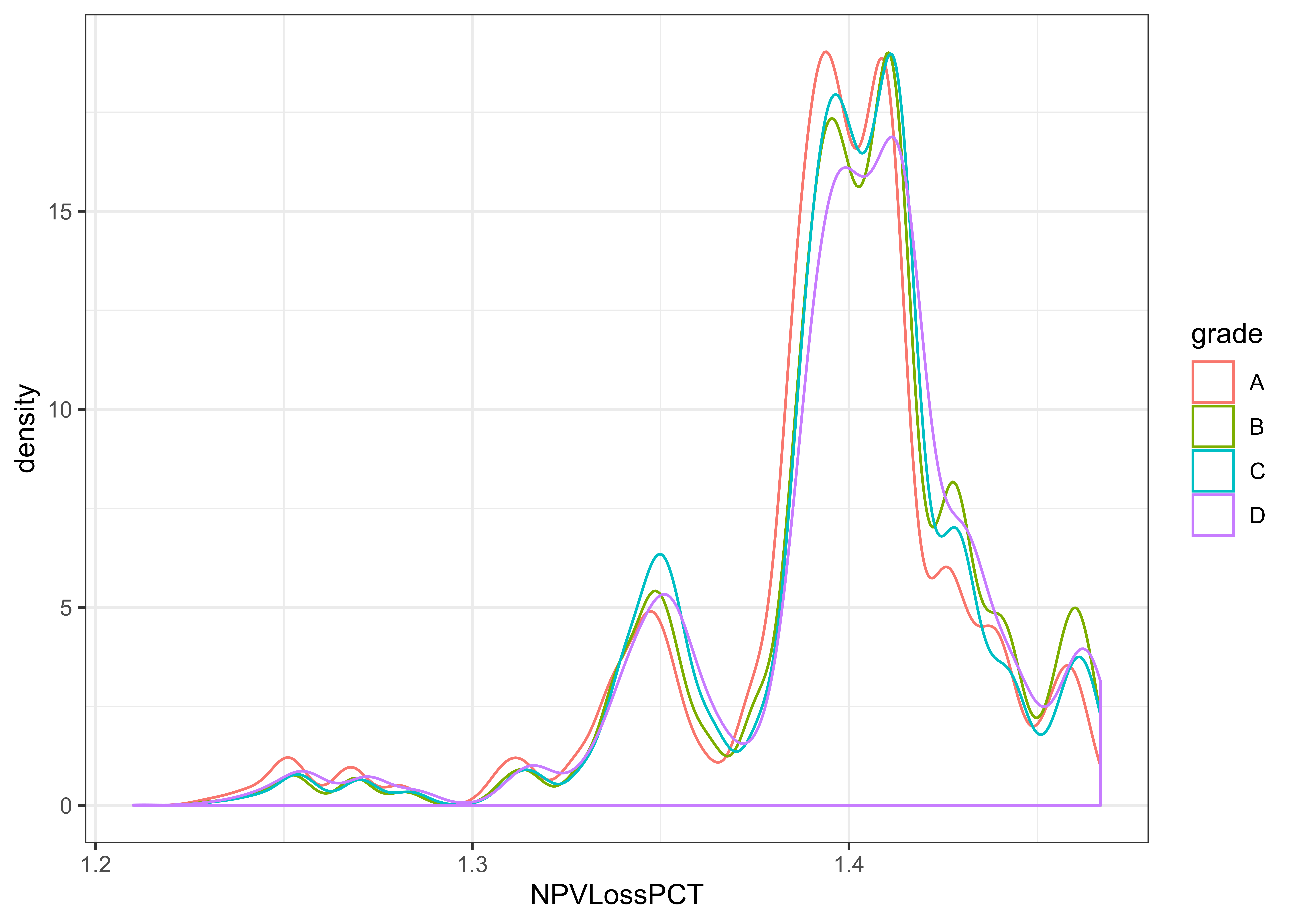
Figure 2.14: NPV % higher than 120% (no y-axis scaling)

• Figure 2.15 and figure 2.16 show a second and third mode around 41% and -1%;

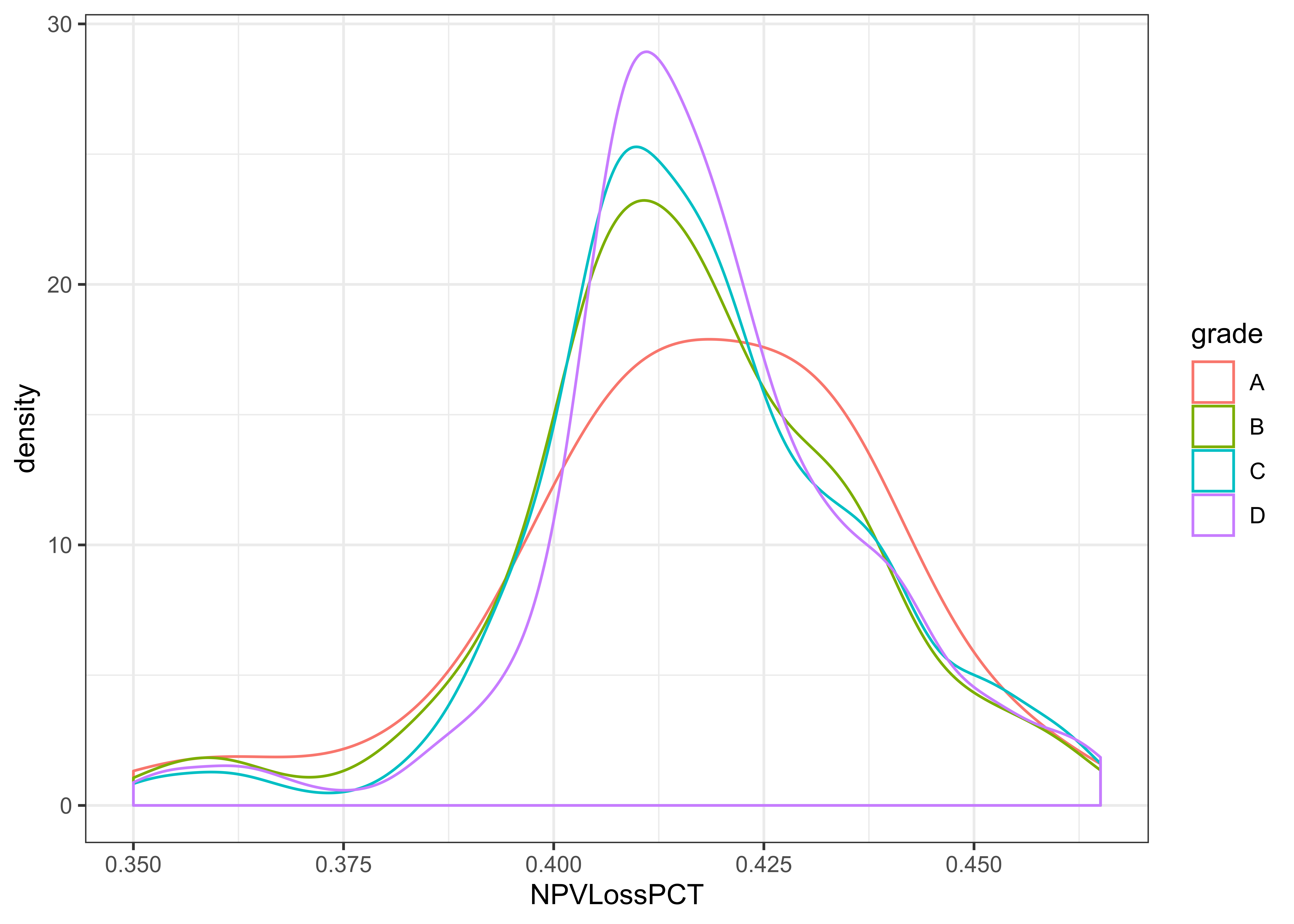
Figure 2.15: NPV % around 41% (no y-axis scaling)

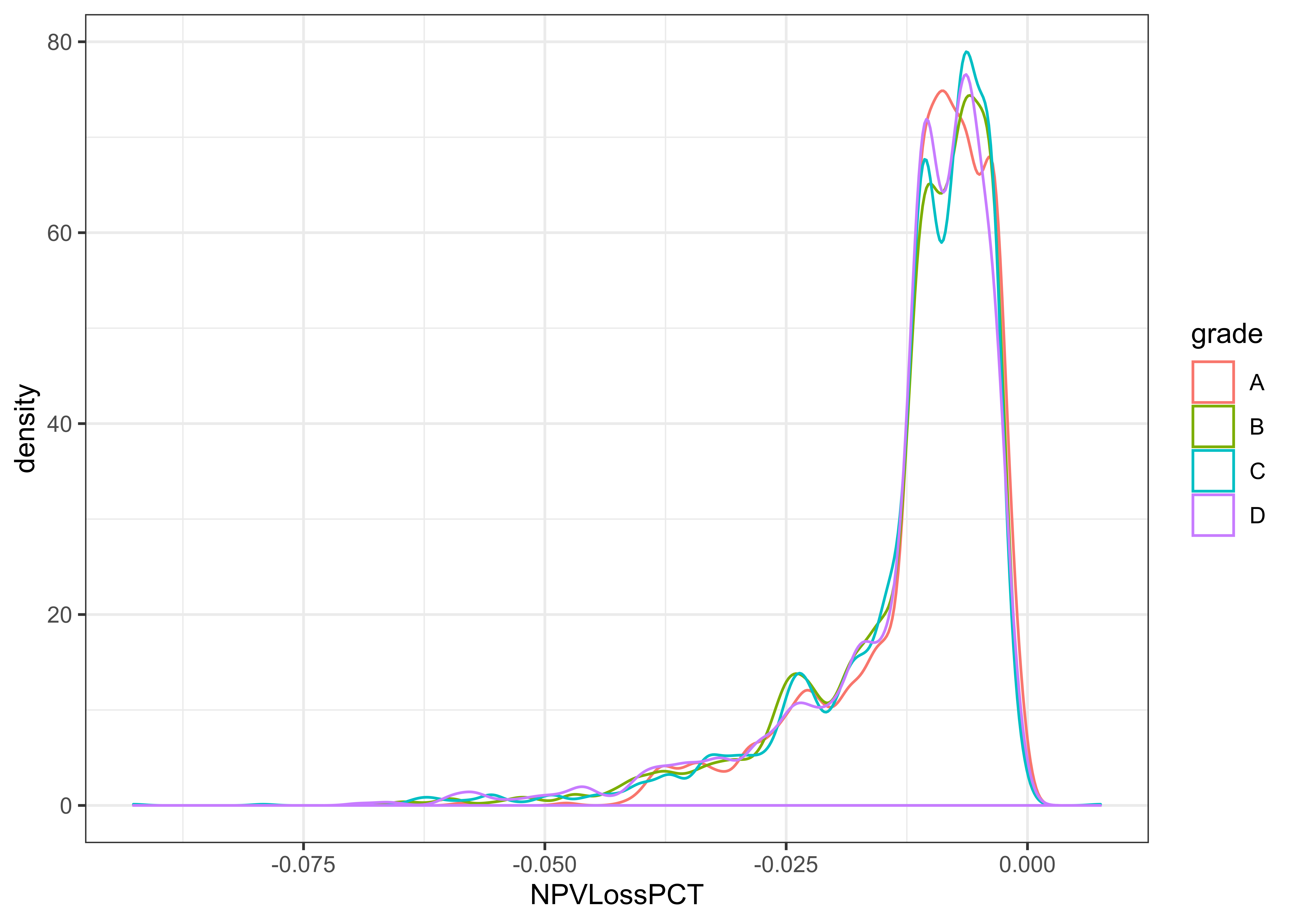
Figure 2.16: NPV % around -1% (no y-axis scaling)

• Finally, figure 2.17 one last very diffuse mode around -100%.

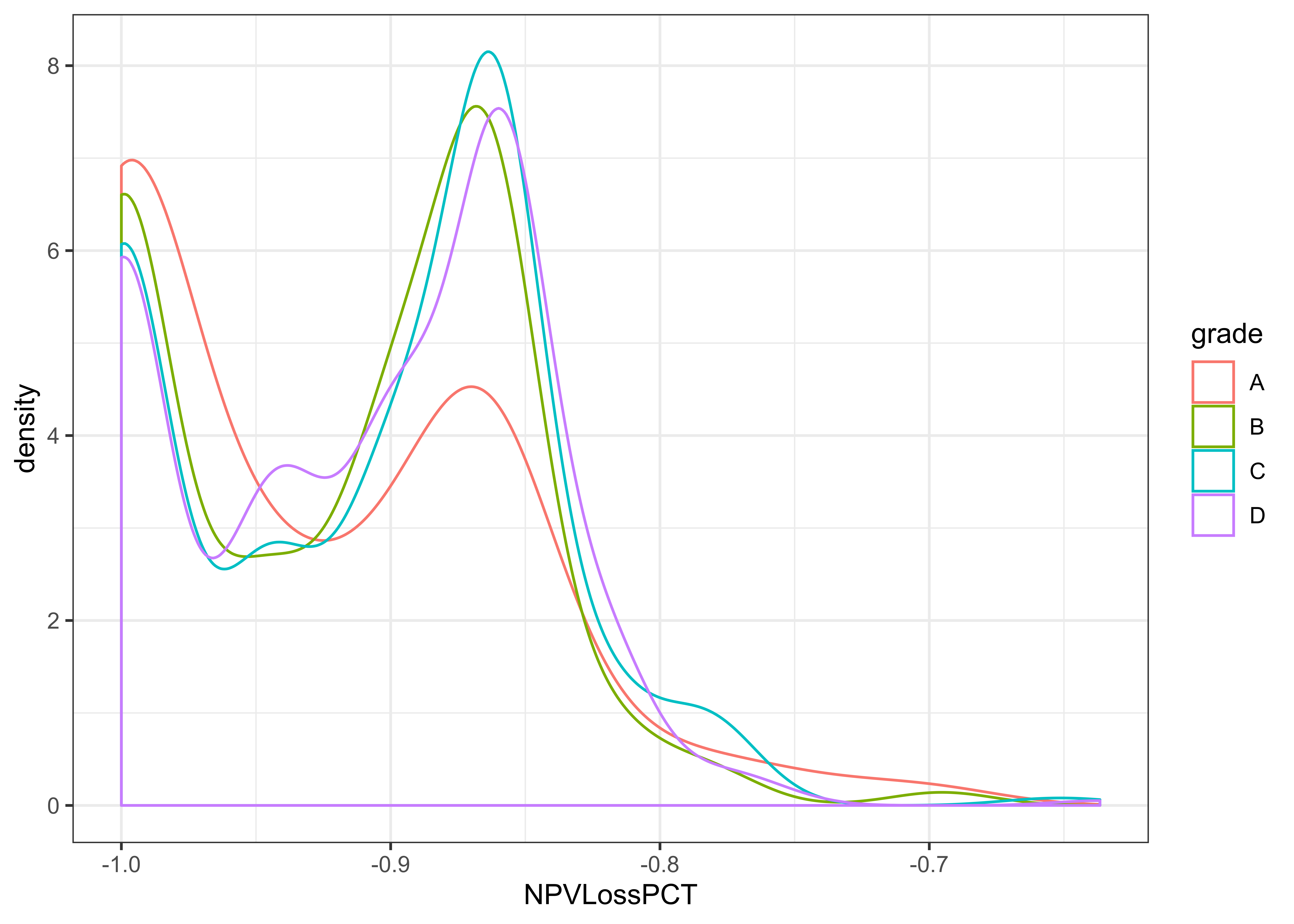
Figure 2.17: NPV % for close to total loss % (no y-axis scaling)

The overall trend is what we should expect. What is surprising is the existence of (1) very clearly defined modes which (2) are common to all types of borrowers. They roughly look log-normal, apart from the mode around 41% which look Gaussian.

2.5 Loan decision

As indicated in the introduction, our focus is on loans that have gone through their entire life cycle to consider their respective pricing, risk and profitability. To that effect, we will remove all loans which are still current (either performing or not), and we will only retain loans which currently available (rated A1 to D5). From here on, everything will be based on this reduced dataset.

This reduced dataset contains 1306356 samples. Most of the loans (ca.80%) have been repaid in full (in other words 1 in 5 loans defaulted). See Table ??.

When grouped by grade (Figure 2.18), we see a clear correlation between grade and default: the lower the grade the higher the portion defaults (note the limited scale with a minimum at about 50%). In addition, in the reduced set most of the business is written in the B- or C-rating range.

Figure 2.18: Funding and Write-offs by Sub-grades

References

Kim, Aleum, and Sung-Bae Cho. 2019. “An Ensemble Semi-Supervised Learning Method for Predicting Defaults in Social Lending.” Engineering Applications of Artificial Intelligence 81. Elsevier: 193–99.

Preparation: Wendy Kan, LendingClub Corporation -. 2019. “Kaggle - LendingClub dataset.” https://www.kaggle.com/wendykan/lending-club-loan-data.

San Francisco - California, LendingClub Corporation -. 2019. “Prospectus Regulatory Filing S3-ASR for Member Payment Dependent Notes.” https://www.sec.gov/Archives/edgar/data/1409970/000140997019000988/0001409970-19-000988-index.htm.

---

7. source: https://en.wikipedia.org/wiki/LendingClub - Retrieval date 15 September 2019↩

8. See LendingClub FAQ at [https://help.lendingclub.com/hc/en-us/articles/215488038] and help page [https://help.lendingclub.com/hc/en-us/articles/216127897-What-happens-when-a-loan-is-charged-off-] ↩

9. See https://www.lendingclub.com/legal/prospectus↩

10. Note that we will add the second and third power of time (measure in months) to create this non-linearity. This will be the only real feature engineering that will be performed on the dataset.↩

11. https://www.lendingclub.com/investing/investor-education/interest-rates-and-fees↩

12. Corporate borrowers would negociate interest margins on a case-by-case basis despite similar risk profiles.↩

13. source: https://www.lendingclub.com/investing/investor-education/interest-rates-and-fees↩

14. See https://www.lendingclub.com/info/demand-and-credit-profile.action↩

15. The averages are not weighted by loan amount since an investor can invest in $25 parcels. Weighting would have been appropriate if investors were instead forced to invest in the whole amount.↩

16. Discounting a cash flow at the IRR gives a nil NPV. Discounting at a higher rate, resp. lower, gives a negative, resp. positive, NPV.↩