1.1 Introduction

Generative models are about learning simple representations of a complex datasets; how to, from a few parameters, generate realistic samples that are similar to a given dataset with similar probabilities of occurence. Those few parameters usually follow simple distributions (e.g. uniform or Gaussian), and are transformed through complex transformations into the more complex dataset distribution. This is an unsupervised procedure which, in a sense, mirrors clustering methods: clustering starts from the dataset and summarises it into few parameters.

Although unsupervised, the result of this learning can be used as a pretraining step in a later supervised context, or where that dataset is a mix of labelled and un-labelled data. The properties of the well-understood starting probability distributions can then help draw conclusions about the dataset’s distribution or generate synthetic datasets.

The same methods can also be used in supervised learning to learn the representation of a target dataset (categorical or continuous) as a transformation of the features dataset. The unsupervised becomes supervised.

What does representation learning actually mean? It is the automatic search for a few parameters that encapsulate rich enough information to generate a dataset. Generative models learn those parameters and, starting from them, how to re-create samples similar to the original dataset.

Let’s use cars as an analogy.

All cars have 4 wheels, an engine, brakes, seats. One could be interested in comfort or racing them or lugging things around or safety or fitting as many kids as possible. Each base vector could be express any one of those characteristics, but they will all have an engine, breaks and seats. The generation function recreates everything that is common. It doesn’t matter if the car is comfy or not; it needs seats and a driving wheel. The generative function has to create those features. However, the exact number of cylinders, its shape, the seats fabric, or stiffness of the suspension all depend on the type of car.

The true fundamentals are not obvious. For a long time, American cars had softer suspension than European cars. The definition of comfortable is relative. The performance of an old car is objectively not the same as compared to new ones. Maybe other characteristics are more relevant to generate. Maybe price? Consumption? Year of coming to market? All those factors are obviously inter-related.

Generative models are more than generating samples from a few fundamental parameters. They also learn what those parameters should be.

1.2 Latent variables

Still using the car analogy, if the year of a model was not given, the generative process might still be able to conclude that the model year should be an implicit parameter to be learned since relevant to generate the dataset: year is an unstated parameter that explains the dataset. Both the Lamborghini Miura and Lamborghini Countach [^1] were similar in terms of perceived performance and exclusivity at the time they were created. But actual performances and styling where incredibly different.

If looking at the stock market: take a set of market prices at a given date; it would have significantly different meanings in a bull or a bear market. Market regime would be a reasonable latent variable.

1.3 Examples of generative models

There are quite a number of generative models. such restricted Boltzmann machines, deep belief networks. Refer to (Theodoridis 2020) and (Russell and Norvig 2020) for example. Let’s consider generative adversarial networks and variational auto-encoders.

1.3.1 Generative Adversarial Networks (GANS)

Recently, GANs have risen to the fore as a way to generate artificial datasets that are, for some definition, indistinguishable from a real dataset. They consist of two parts:

Figure 1.1: Generative Adversarial Networks (source: (Hitawala 2018)))

• A generator which is the generative model itself: given a simple representation, the generator proposes samples that aim to be undistinguishable from the dataset sample.

• A discriminator whose job is to identify whether a sample comes from the generator or from the dataset.

Both are trained simultaneously:

• if the discriminator finds it obvious to guess, the generator is not doing a good job and needs to improve;

• if the discriminator guesses 50/50 (does no better than flipping a coin), it has to discover which true dataset features are truly relevant.

1.3.2 Variational autoencoders

A successful GAN can replicate the richness of a dataset, but not its probability distribution. A GAN can generate a large number of correct sentences, but will not tell how likely to occur that sentence is (or at least guarantee that the distributions match). ‘The dog chases the cat’ and ‘The Chihuahua chases the cat’ are both perfectly valid, but the latter less unlikely to appear.

Generally speaking, autoencoders learn an encoder that takes a sample to generate a vector in a latent space, and a decoder that generates samples from latent state variables. The encoder and the decoder really mirror each other. However, this general approach does not learn how to sample from the latent space. Sampling randomly from the latent space may generate perfectly valid data (i.e. very similar to that in the training dataset), but the distribution of a generated datasest and the training dataset would likely be very different. This is the same problem GANs face.

Figure 1.2: Variational Auto-Encoder (source: Shenlong Wang)

Variable autoencoders (VAEs) take another approach. Instead of just learning a function representing the data, they learn the parameters of a probability distribution representing the data. We can then sample from the distribution and generate new input data samples. The decoder and the encoder are trained simultaneously on the dataset samples, proposing a generated sample from that projection and training on the reconstruction loss. The encoder actually learns means and standard deviations of the each latent variable, each being a normal distribution. The samples generated will be as rich as the GAN’s, but the probability of a sample being generated will depend on the learned distributions.

See (Kingma and Welling 2019) for an approachable extensive introduction. The details include implementation aspects (in particular the reparametrisation trick) that are critical to the success of this approach.

1.4 Limitations

We limited the introduction to those two techniques to merely highlight two fundamental aspect that generative models aim at:

• find a simple representation;

• explore and replicate the richness of the dataset;

• replicate the probability distribution of the dataset.

Note that depending on the circumstances, the last aim may not necessarily be important.

As usual, training and optimisation methods are at risk of getting stuck at local optima. In the case of those two techniques, this manifests itself in different ways:

• GANs Mode collapse: Mode collapse occurs in GANs when the generator only explores limited domains. Imagine training a GAN to recognise mammals (the dataset would contain kangaroos, whales, dogs and cats…). If the generator proposes everything but kangaroos, it is still properly generate mammals, but obviously misses out on a few possibilities. Essentially, the generator reaches a local minimum where a vanishing gradient becomes too small to explore alternatives. This is in part due to the difficulty of progressing the training of both the generator and the discriminator in a way that does not lock any one of them in a local optimum while the other still needs improving: if either converges too rapidly, the other will struggle to catch up.

• VAEs Posterior collapse: Posterior collapse in VAEs arises when the generative model learns to ignore a subset of the latent variables (although the encoder generates those variables) (Lucas et al. 2019). This happens when (1) a subset of the latent variable space is good enough to generate a reasonable approximation of the dataset and its distribution, and (2) the loss function does not yield large enough gradients to explore other latent variables to further improve the encoder. (More technically, it happens when the variational distribution closely matches the uninformative prior for a subset of latent variables (Tucker et al. 2019).) The exact reasons for this are not entirely understood and this remains an active area of research (refer this extensive list of papers on the topic).

In the next section, we will get into another approach called Normalising Flows which, as we will see, address those two difficulties. Intuitively:

• Mode collapse reflects that the generative process does not generate enough possibilities; that the spectrum of possibilities is not as rich as that of the dataset. Normalising flows attempt to address this in two ways. Firstly, their optimising process aims at optimising (and matching) the amount of information captured by the learned representation to that of the dataset (in the sense of information theory). Secondly, we will see that normalising flows allow to start from a sample in the dataset, flow back to the simple distribution and estimate how (un)likely the generative model would have generated this sample.

• The posterior collapse could simply be a mismatch between the number of latent variables and the dimensionality of the dataset. As we will see, normalising flows impose that the generative model be a bijection which takes away the choice of of a number of dimensions (although this shifts the issue to become one of parameters regularisation).

On a final note, it will not be surprising that GANs and VAEs have been combined (see (Larsen et al. 2016)).

2.1 Introduction

One important limitations of the approaches described above is that the generation/decoding flow is unidirectional: one starts from a source distribution, sometimes with well-known properties, and generates a richer target distribution. However, given a particular sample in the target distribution, there is no guaranteed way to identify where it would fall in the latent space distribution. That flow of transformation from source to target is not guaranteed to be bijective or invertible (same meaning, different crowds).

Normalising flows are a generic solution to that issue: it is a transformation from a simple distribution (e.g. uniform or normal) to a more complex distribution by an invertible and differentiable mapping, where the probability density of a sample can be evaluated by transforming it back to the original distribution. The density is evaluated by computing the density of the normalised inverse-transformed sample. The word normalising refers to the normalisation of the transformation, and not to the fact that the original distribution could be normal.

In practice, this is a bit too general to be of any use. Let’s break this down:

• The original distribution is simple with well-known statistical properties: i.i.d. Gaussian or uniform distributions.

• The transformation function is expected to be complicated, and is normally specified as a series of successive transformations, each simpler (though expressive enough) and easy to parametrise.

• Each simple transformation is itself invertible and differentiable, therefore guaranteeing that the overall transformation is too.

• We want the transformation to be normalised: the cumulative probability density of the generated targets from latent variables has to be equal 1. Otherwise, flowing backwards to use the properties of the original would make no sense.

Figure 2.1: Normalizing Flows (Source: (Rezende and Mohamed 2016))

• Geometrically, the probability distribution around each point in the latent variables space is a small volume that is successively transformed with each transformation. Keeping track of all the volume changes ensures that we can relate probability density functions in the original space and the target space.

• How to keep track? This is where the condition of having invertible and differentiable transformation becomes important. (Math-speak: we have a series of diffeomorphisms which are transformations from one infinitesimal volume to another. They are invertible and differentiable, and their inverses are also differentiable.) If one imagines that small volume of space around a starting point, that volume gets distorted along the way. At each point, the transformation is differentiable and can be approximated by a linear transformation (a matrix). That matrix is the Jacobian of the transformation at that point (diffeomorphims also means that the Jacobian matrix exists and is invertible). Being invertible, the matrix has no zero eigenvalues and the change of volume is locally equal to the product of all the eigenvalues (more precisely, their absolute values): the volume gets squeezed along some dimensions, expanded along others. Rotations are irrelevant. The product of the eigenvalues is the determinant of the matrix. A negative eigenvalue would mean that the infinitesimal volume is ‘flipped’ along that direction. That sign is irrelevant: the local volume change is therefore the absolute value of the determinant.

• We can already anticipate a computation nightmare: determinants are computationally very heavy. Additionally, in order to backpropagate a loss to optimise the transformations’ parameters, we will need the Jacobians of the inverse transformations (the inverse of the transformation Jacobian). Without further simplifying assumptions or tricks, normalising flows would be impractical for large dimensions.

2.2 Short example

We will use examples from the Torchdyn library. Torchdyn builds on Pytorch and the polish of the Pytorch Lightning library which streamlines a lot of the Pytorch boilerplate.

In this example, we try to model a dataset distribution which is the superposition of 6 bivariate normal distribution centred on the summits of an hexagon. The idea is to learn how to map and transform a simple distribution (a simple bivariate normal distribution) into that distribution with 6 modes.

import sys 

import matplotlib.pyplot as plt

# Pytorch provides the autodifferentation and the neural networks
import torch
import torch.utils.data as data
from torch.distributions import MultivariateNormal

import torchdyn
from torchdyn.models import CNF, NeuralDE, REQUIRES_NOISE
from torchdyn.datasets import ToyDataset

import pytorch_lightning.core.lightning as pl

device = torch.device("cuda" if torch.cuda.is_available() else "cpu")

using Random, Distributions, Plots, GR, LinearAlgebra

# Getting ready for GPUs is OK given the automatic fallback to CPU
using CUDA

2.2.2 Dataset

For this simple example, we will work with several Gaussians each centred on a hexagon.

2.2.2.1 Python version

# The dataset has about 16k samples
n_samples = 1 << 14

# That will be spread across 6 Gaussians on a plave. 
n_gaussians = 6

# Torchdyn has a helper funciton to generate the dataset.
X, yn = ToyDataset().generate(n_samples // n_gaussians, 
                              'gaussians', 
                              n_gaussians=n_gaussians, 
                              std_gaussians=0.5, 
                              radius=4, dim=2)

# Z-score the generated dataset.
X = (X - X.mean())/X.std()

# Let's look what we have
plt.figure(figsize=(5, 5))
plt.scatter(X[:,0], X[:,1], c='black', alpha=0.2, s=1.)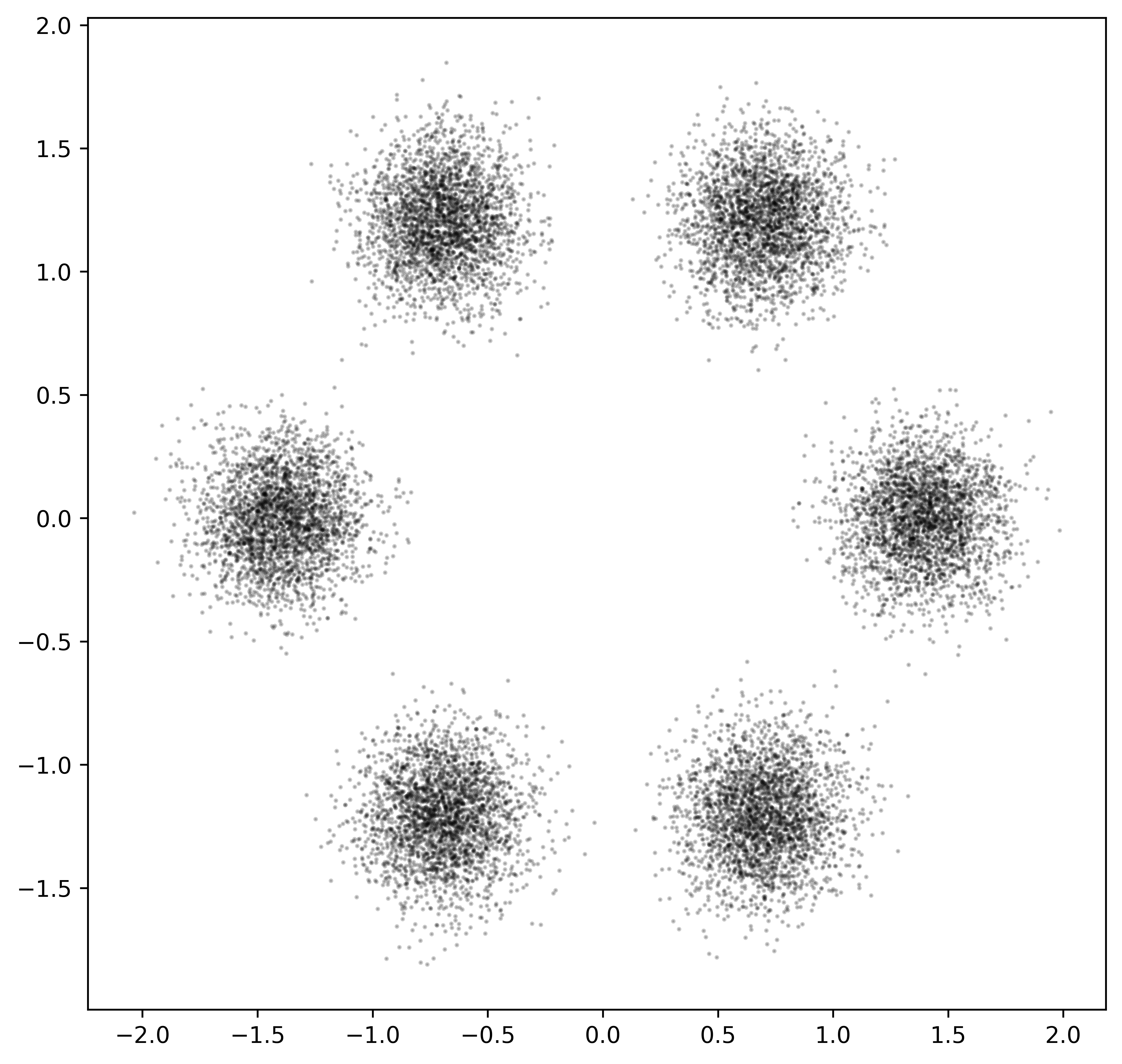

Figure 2.2: Toy dataset

2.2.2.2 Julia version

# The Julia version closely follows the Python one but we do not have the benefit of the helper function.

n_samples = 1 << 14
n_gaussians = 6
n_dims = 2

t_span = (0., 1.)
t_steps = 50

x_span = y_span = -2.5:0.1:2.5

X_span = repeat(x_span', length(y_span), 1)
Y_span = repeat(y_span,  1,              length(x_span))


function generate_gaussians(; n_dims = n_dims, n_samples=100, n_gaussians=7, 
        radius=1.f0, std_gaussians=0.2f0, noise=0.001f0)

    x = zeros(Float64, n_dims, n_samples * n_gaussians)
    y = zeros(Float64, n_samples * n_gaussians)
    incremental_angle = 2 * π / n_gaussians
    
    dist_gaussian = MvNormal(n_dims, sqrt(std_gaussians))

    if n_dims > 2
        dist_noise = MvNormal(n_dims - 2, sqrt(noise))
    end
    
    current_angle = 0.f0
    for i ∈ 1:n_gaussians
        current_loc = zeros(Float32, n_dims, 1)
        if n_dims >= 1
            current_loc[1] = radius * cos(current_angle)
        end
        
        if n_dims >= 2
            current_loc[2] = radius * sin(current_angle)
        end
        
        x[1:n_dims, (i-1)*n_samples+1:i*n_samples] = current_loc[1:n_dims] .+ rand(dist_gaussian, n_samples)
        if n_dims > 2
            x[1:n_dims-2, (i-1)*n_samples+1:i*n_samples] = rand(noise, n_samples)
        end
        
        
        y[   (i-1)*n_samples+1:i*n_samples] = Float32(i) .* ones(Float32, n_samples)
        
        current_angle = current_angle + incremental_angle
    end
    
    return Float64.(x), Float64.(y)
end


X, Y = generate_gaussians(; n_samples = n_samples ÷ n_gaussians, 
                            n_gaussians = n_gaussians, 
                            radius = 4.0f0, 
                            std_gaussians = 0.5f0)
X = (X .- mean(X)) ./ std(X)
X_SIZE = size(X)[2]


# We will continue onward using the Plotly backend
plotly() 
if n_dims == 1
    histogram(X[1, :], title = "Sample from the true density")
else
    scatter!(X[1, :], X[2, :], title = "Sample from the true density", markershape=:cross, markersize=1)
end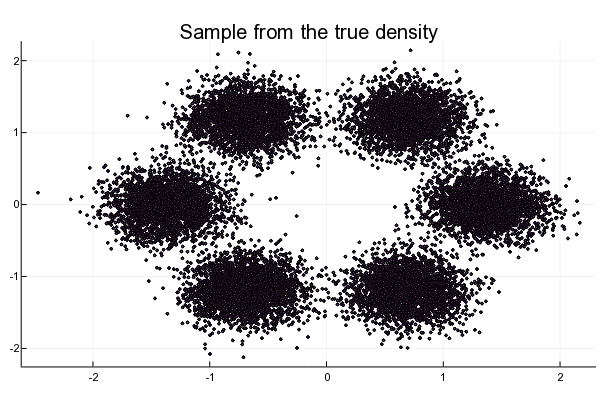

Figure 2.3: Toy dataset

X_train = torch.Tensor(X).to(device)
y_train = torch.LongTensor(yn).long().to(device)

train = data.TensorDataset(X_train, y_train)
trainloader = data.DataLoader(train, batch_size=1024, shuffle=True)

# Continuous Normalisising Flows require an estimate of the trace of the Jacobian matrix. 
# This will be explained further down.
def autograd_trace(x_out, x_in, **kwargs):
    """Standard brute-force means of obtaining trace of the Jacobian, O(d) calls to autograd"""
    trJ = 0.
    for i in range(x_in.shape[1]):
        trJ += torch.autograd.grad(x_out[:, i].sum(), x_in, allow_unused=False, create_graph=True)[0][:, i]
    return trJ

# Continuous Normalisising Flows 
class CNF(nn.Module):
    def __init__(self, net, trace_estimator=None, noise_dist=None):
        super().__init__()

        self.net = net
        self.noise_dist, self.noise = noise_dist, None

        self.trace_estimator = trace_estimator if trace_estimator is not None else autograd_trace;
        if self.trace_estimator in REQUIRES_NOISE:
            assert self.noise_dist is not None, 'This type of trace estimator requires specification of a noise distribution'

    def forward(self, x):
        with torch.set_grad_enabled(True):
            # first dimension reserved to divergence propagation
            x_in = torch.autograd.Variable(x[:,1:], requires_grad=True).to(x) 
            
            # the neural network will handle the data-dynamics here
            x_out = self.net(x_in)

            trJ = self.trace_estimator(x_out, x_in, noise=self.noise)
        
        # `+ 0*x` has the only purpose of connecting x[:, 0] to autograd graph
        return torch.cat([-trJ[:, None], x_out], 1) + 0*x 

f = nn.Sequential(
        nn.Linear(2, 64),
        nn.Softplus(),
        nn.Linear(64, 64),
        nn.Softplus(),
        nn.Linear(64, 64),
        nn.Softplus(),
        nn.Linear(64, 2),
    )

# cnf wraps the net as with other energy models
# default trace_estimator, when not specified, is autograd_trace
cnf = CNF(f, trace_estimator=autograd_trace)
nde = NeuralDE(cnf, solver='dopri5', s_span=torch.linspace(0, 1, 2), sensitivity='adjoint', atol=1e-4, rtol=1e-4)

multi_gauss_model = nn.Sequential(Augmenter(augment_idx=1, augment_dims=1), nde).to(device)

using DiffEqFlux, Optim, OrdinaryDiffEq, Zygote, Flux, JLD2, Dates, Serialization

# The NN is defined with the Flux package. 32 neurons per dimensions.
f = Chain(Dense(n_dims, 32 * n_dims, tanh), 
          Dense(32 * n_dims, 32 * n_dims, tanh), 
          Dense(32 * n_dims, 32 * n_dims, tanh), 
          Dense(32 * n_dims, n_dims)) |> gpu


# The CNF is defined as a differential equation AND the method used for its optimisation (FFJORD)
cnf_ffjord = FFJORD(f, t_span, Tsit5(), basedist = MvNormal(n_dims, 1.), monte_carlo = true)

# The optimisation will be to maximise the negative log loss  
function loss_adjoint(θ)
    logpx = cnf_ffjord(X, θ)[1]
    return -mean(logpx)[1]
end

multi_gauss_prior = MultivariateNormal(torch.zeros(2).to(device), torch.eye(2).to(device))

class LearnerMultiGauss(pl.LightningModule):
    
    def __init__(self, model:nn.Module):
        super().__init__()
        
        self.model = model
        self.iters = 0

    
    def forward(self, x):
        return self.model(x)

    
    def training_step(self, batch, batch_idx):
        self.iters += 1
        x, _ = batch
        xtrJ = self.model(x)
        logprob = multi_gauss_prior.log_prob(xtrJ[:,1:]).to(x) - xtrJ[:,0] # logp(z_S) = logp(z_0) - \int_0^S trJ
        loss = -torch.mean(logprob)
        nde.nfe = 0
        return {'loss': loss}

    
    def configure_optimizers(self):
        return torch.optim.AdamW(self.model.parameters(), lr=2e-3, weight_decay=1e-5)

    
    def train_dataloader(self):
        return trainloader

learn = LearnerMultiGauss(multi_gauss_model)
trainer = pl.Trainer(max_epochs=300)
trainer.fit(learn)

# First define a callback function that will keep a record of losses and plot the learned distribution
callback = function(params, loss)
    
    store_all = true
    store_loss = false
    store_plot = false
    
    global iter += 1
    
    # Print the current loss
    println("Iteration $iter  -- Loss: $loss")
    
    
    # Keep a record of everything

    if store_all || store_loss
        push!(losses, loss)
    end
        
    if store_all || store_plot
        # Plot the transformation
        vals = map( (x, y) -> cnf_ffjord([x, y], params; monte_carlo=false)[1][], 
                    X_span, Y_span)    
    
        p = Plots.contour(x_span, y_span, vals, fill=true)
        p
        push!(list_plots, p)
    
        push!(min_maxes, 
              (minimum(vals), maximum(vals)))
    end
        
    return false
end


# Train using the ADAM optimizer. 

# List accumulators for the results
iter = 0; list_plots = []; min_maxes = []; losses = []

res1 = DiffEqFlux.sciml_train(
        loss_adjoint, 
        cnf_ffjord.p,
        ADAM(0.002), 
        cb = callback,
        maxiters = 100)

2.2.8 Sampling

2.2.8.1 Python version

We can now sample from the independent Gaussians to see what is generated from them.

# Let's draw 16k samples
sample = multi_gauss_prior.sample(torch.Size([n_samples]))

# integrating from 1 to 0
multi_gauss_model[1].s_span = torch.linspace(1, 0, 2)
new_x = multi_gauss_model(sample).cpu().detach()
sample = sample.cpu()

plt.figure(figsize=(12, 4))

plt.subplot(121)
plt.scatter(new_x[:,1], new_x[:,2], s=2.3, alpha=0.2, linewidths=0.3, c='blue', edgecolors='black')
plt.xlim(-2, 2) ; plt.ylim(-2, 2)
plt.title('Samples')

plt.subplot(122)
plt.scatter(X[:,0], X[:,1], s=2.3, alpha=0.2, c='red',  linewidths=0.3, edgecolors='black')
plt.xlim(-2, 2) ; plt.ylim(-2, 2)
plt.title('Data')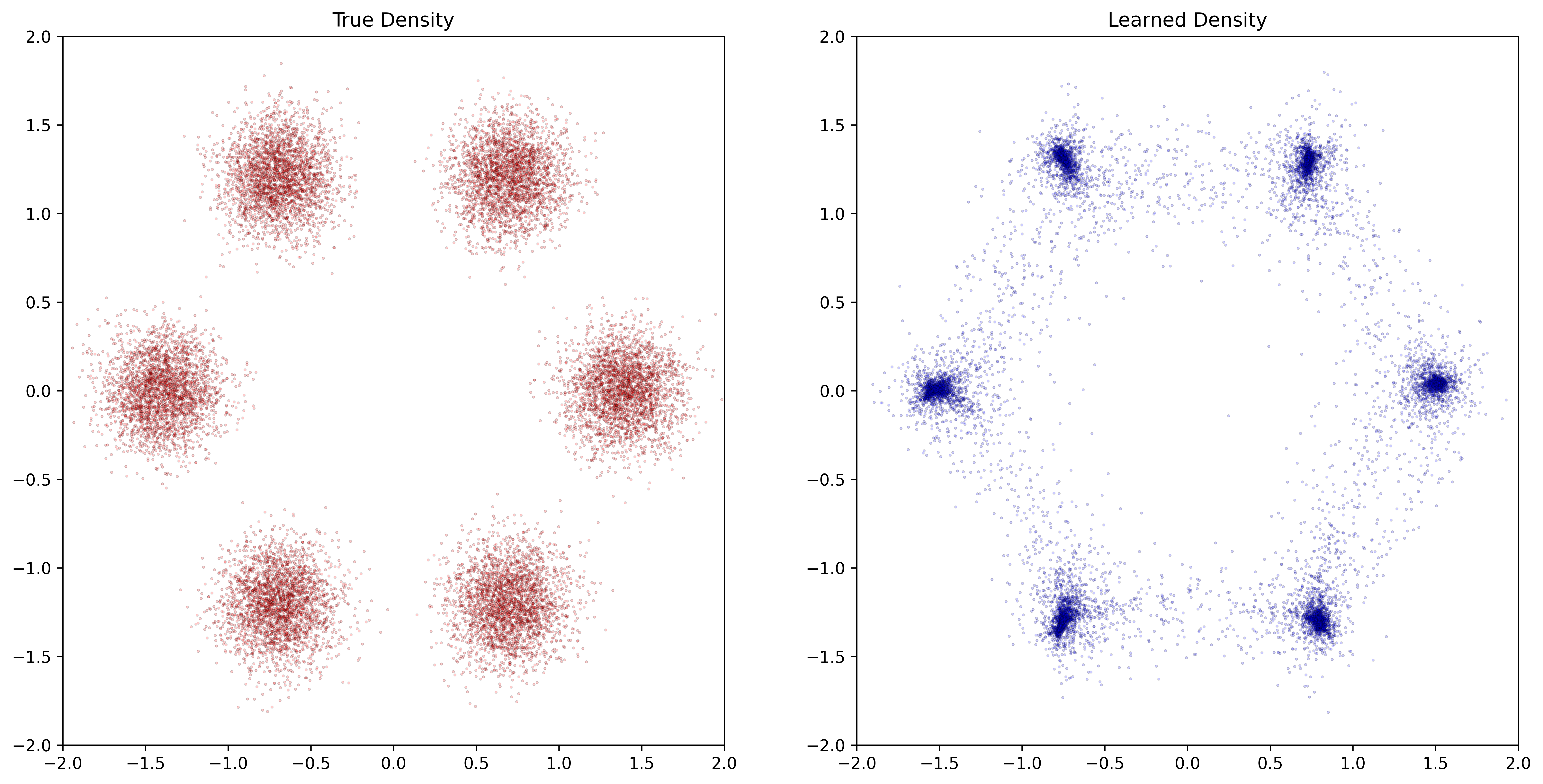

Figure 2.4: Training result

trajectories = model[1].trajectory(Augmenter(1, 1)(sample.to(device)), s_span=torch.linspace(1,0,100)).detach().cpu()

trajectories = trajectories[:, :, 1:] # scrapping first dimension := jacobian trace

n = 1000
plt.figure(figsize=(6, 6))

# Plot the sample
plt.scatter(sample[:n, 0],   sample[:n, 1],   s=4,  alpha=0.8, c='red')

# Dram a line from the sample to the generated data
plt.scatter(trajectories[:,:n, 0],   trajectories[:,:n, 1],   s=0.2, alpha=0.1, c='olive')

# Plot the generated data
plt.scatter(trajectories[-1, :n, 0], trajectories[-1, :n, 1], s=4,   alpha=1.0, c='blue')

plt.legend(['Prior sample z(S)', 'Flow', 'z(0)'])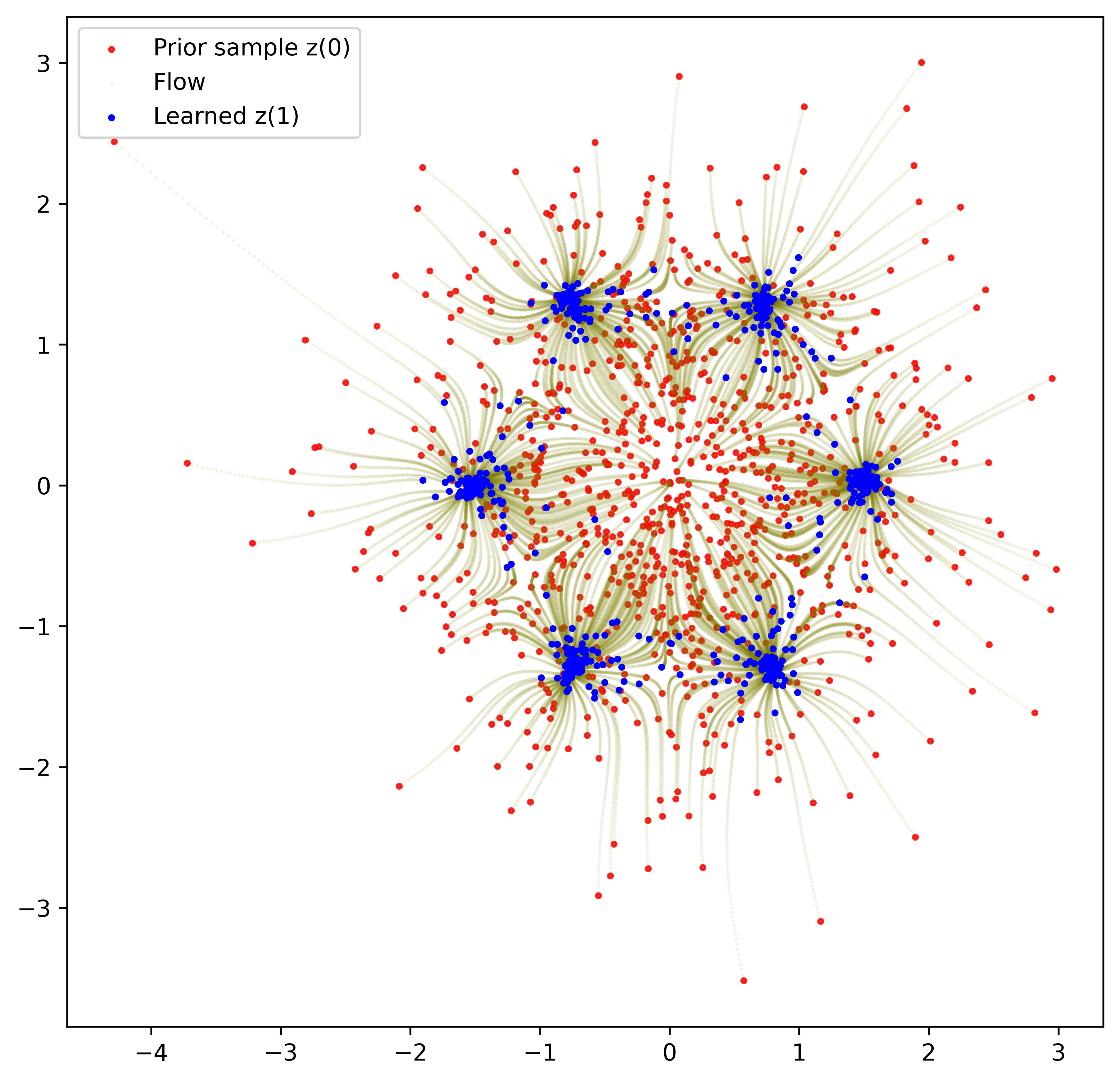

Figure 2.5: Flows

We can see that the flow is smooth having sampled 1,000 points. For each sampled point in red), we trace its flow (in olive) to its final destination (in blue). The initial sample follows a 2D Gaussian and sort of explodes towards the direction of each mode. It is important to emphasise how economical this is in terms of parameters. We have become accustomed to deep learning networks with a staggering numbers of cascaded layers, each with its parameters to be optimised. This Neural ODE is a single perceptron with 2 hidden layers that is applied an infinite numbers of times (within the approximation of the ODE solver).

2.2.8.2 Julia version

We plot the progress of the 100 iterations:

anim = @animate for i ∈ 1:length(list_plots)
    # Necessary to create a new plot for each frame
    Plots.plot(1)
    Plots.plot!(list_plots[i])
end

gif(anim) # GIF converted to mp4 to reduce animation file size

2.3 Into the maths

The starting distribution is a random variable \(X\) with a support in \(\mathbb{R}^D\). For simplicity, we will assume just assume that the support is \(\mathbb{R}^D\) since using measurable supports does not change the results. If \(X\) is transformed into \(Y\) by an invertible function/mapping \(f: \mathbb{R}^D \rightarrow \mathbb{R}^D\) (\(Y=f(X)\)), then the density function of \(Y\) is:

\[ \begin{aligned} P_Y(\vec{y}) & = P_X(\vec{x}) \left| \det \nabla f^{-1}(\vec{y}) \right| \\ & = P_X(\vec{x}) \left| \det\nabla f(\vec{x}) \right|^{-1} \end{aligned} \]

where \(\vec{x} = f^{-1}(\vec{y})\) and \(\nabla\) represents the Jacobian operator. Note the use of \(\vec{x}\) to denote vectors instead of the usual \(\mathbf{x}\) which on-screen is easily read as a scalar.

Following the direction of \(f\) is the generative direction; following the direction of \(f^{-1}\) is the normalising direction (as well as being the inference/encoding direction in the context of training).

If \(f\) were a series of individual transformation \(f = f_N \circ f_{N-1} \circ \cdots \circ f_1\), then it naturally follows that:

\[ \begin{aligned} \det\nabla f(\vec{x}) & = \prod_{i=1}^N{\det \nabla f_i(\vec{x}_i)} \\ \det\nabla f^{-1}(\vec{x}) & = \prod_{i=1}^N{\det \nabla f_i^{-1}(\vec{x}_i)} \end{aligned} \]

In order to make clear that the Jacobian is not taken wrt the starting latent variables \(x\), we use the notation:

\[ \vec{x}_i = f_{i-1}(\vec{x}_{i-1}) \]

2.4 Training loss optimisation and information flow

Before moving into examples of normalising flows, we need to comment on the loss function optimisation. How do we determine the generative model’s parameters so that the generated distribution is as close as possible to the real distribution (or at least to the distribution of the samples drawn from that true distribution)?

A standard way to do this is to calculate the Kullback-Leibler divergence between the two. Recall that the KL divergence \(\mathbb{KL}(P \vert \vert Q)\) is not a distance as it is not symmetric. I personally read \(\mathbb{KL}(P \vert \vert Q)\) as “the loss of information on the true \(P\) if using the approximation \(Q\)” as a way to keep the two distributions at their right place (writing \(\mathbb{KL}(P_{true} \vert \vert Q_{est.})\) will help clarify the proper order).

The KL divergence is defined as:

\[ \begin{aligned} \mathbb{KL}(P_{true} \vert \vert Q_{est.}) = \mathbb{E}_{P_{true}(\vec{x})} \left[ \log \frac{P_{true}(\vec{x})}{Q_{est.}(\vec{x})} \right] \end{aligned} \]

Or for a discrete distribution:

\[ \begin{aligned} \mathbb{KL}(P_{true} \vert \vert Q_{est}) & = \sum_{\vec{x} \in X} P_{true}(\vec{x}) \log \frac{P_{true}(\vec{x})}{Q_{est}(\vec{x})} \\ & = \sum_{\vec{x} \in X} P_{true}(\vec{x}) \left[ \log P_{true}(\vec{x}) - \log Q_{est}(\vec{x}) \right] \end{aligned} \]

In our particular case, this becomes:

\[ \begin{aligned} \mathbb{KL}(P_{true} \vert \vert P_Y) & = \sum_{\vec{x} \in X} {P_{true}(\vec{x}) \log \frac{P_{true}(\vec{x})}{P_Y(\vec{y})}} \\ & = \sum_{\vec{x} \in X} {P_{true}(\vec{x}) \left[ \log P_{true}(\vec{x}) - \log P_Y(\vec{y}) \right] } \end{aligned} \]

Recalling that we have a transformation from \(\vec{x}\) to \(\vec{y}\):

\[ \begin{aligned} P_Y(\vec{y}) & = P_X(\vec{x}) \left| det \nabla f^{-1}(\vec{y}) \right| \\ & = P_X(\vec{x}) \left| det\nabla f(\vec{x}) \right|^{-1} \end{aligned} \]

We end up with:

\[ \mathbb{KL}(P_{true} \vert \vert P_Y) = \sum_{\vec{x} \in X} {P_{true}(\vec{x}) \left[ \log P_{true}(\vec{x}) - \log \left( P_X(\vec{x}) \left| det \nabla f(\vec{x}) \right|^{-1} \right) \right] } \]

Minimising this divergence is achieved by changing the parameter which generate \(f\).

The divergence is one of many loss formulae that can be used to measure the distance (in the loose sense of the word) between the true and generated distributions. But the KL divergence illustrates how logarithms of the probability distributions naturally appear. Another common formulation of the loss is the Wasserstein distance.

In the setting of the normalising flows (and VAEs), we have two transformations: the inference direction (the encoder) and the generative direction (the decoder). Given the back-and-forth nature, it makes sense to not favour one direction over the other. Instead of using the KL divergence which is not symmetric, we can use the mutual information (this is equivalent to using free energy as in (Rezende and Mohamed 2016)).

Regardless of the choice of loss function, it is obvious that optimising \(\mathbb{KL}(P_{true} \vert \vert P_Y)\) cannot be contemplated without serious optimisations. Finding more tractable alternative distance measurements is an active research topic.¹

2.5 Basic flows

In their paper, (Rezende and Mohamed 2016) experimented with simple transformations: a linear transformation (with a simple non-linear function) called planar flows and flows within a space centered on a reference latent variable called radial flows.

2.5.2 Planar flow example

This is an example inspired by https://github.com/abdulfatir/planar-flow-pytorch.

2.5.2.1 Imports

# https://github.com/abdulfatir/planar-flow-pytorch

%matplotlib inline

import matplotlib.pyplot as plt
import numpy as np

import torch
import torch.nn as nn
device = torch.device("cuda" if torch.cuda.is_available() else "cpu")

from tqdm.notebook import tqdm

2.5.2.2 Constants and parameters

# Constants

# Size of a layer. We operate on a plane => 2D
n_dimensions = 2

# Number of layers
n_layers = 16

# Number of samples drawn
n_samples = 500

2.5.2.3 Densities to be learned

# Unnormalized Density Functions

# As a torch object for training
def true_density(z):
    z1, z2 = z[:, 0], z[:, 1]
    norm = torch.sqrt(z1 ** 2 + z2 ** 2)
    exp1 = torch.exp(-0.5 * ((z1 - 2) / 0.8) ** 2)
    exp2 = torch.exp(-0.5 * ((z1 + 2) / 0.8) ** 2)
    u = 0.5 * ((norm - 4) / 0.4) ** 2 - torch.log(exp1 + exp2)
    return torch.exp(-u)

# As a Numpy object for plotting
def true_density_np(z):
    z1, z2 = z[:, 0], z[:, 1]
    norm = np.sqrt(z1 ** 2 + z2 ** 2)
    exp1 = np.exp(-0.5 * ((z1 - 2) / 0.8) ** 2)
    exp2 = np.exp(-0.5 * ((z1 + 2) / 0.8) ** 2)
    u = 0.5 * ((norm - 4) / 0.4) ** 2 - np.log(exp1 + exp2)
    return np.exp(-u)

figure, axes = plt.subplots(1, 1, figsize=(8, 8))

# True Density
x = np.linspace(-5, 5, 500)
y = np.linspace(-5, 5, 500)

X, Y = np.meshgrid(x, y)

data = np.vstack([X.flatten(), Y.flatten()]).T

# Unnormalized density
density = true_density_np(data) 

axes.pcolormesh(X, Y, density.reshape(X.shape), cmap='Blues', shading='auto')
axes.set_title('True density')
axes.axis('square')
axes.set_xlim([-5, 5])
axes.set_ylim([-5, 5])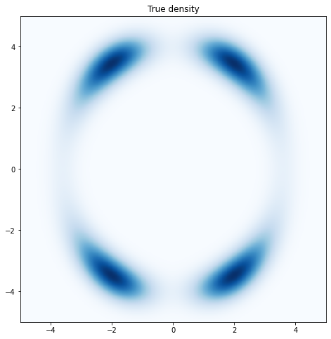

Figure 2.6: True density

2.5.2.4 Definition of a single layer

class PlanarTransform(nn.Module):
    def __init__(self, dim=2):
        super().__init__()
        
        self.u = nn.Parameter(torch.randn(1, dim) * 0.01)
        self.w = nn.Parameter(torch.randn(1, dim) * 0.01)
        self.b = nn.Parameter(torch.randn(()) * 0.01)
    
    def m(self, x):
        return -1 + torch.log(1 + torch.exp(x))
    
    def h(self, x):
        return torch.tanh(x)
    
    def h_prime(self, x):
        return 1 - torch.tanh(x) ** 2
    
    def forward(self, z, logdet=False):
        # z.size() = batch x dim
        u_dot_w = (self.u @ self.w.t()).view(())
        
        # Unit vector in the direction of w
        w_hat = self.w / torch.norm(self.w, p=2) 
        
        # 1 x dim
        u_hat = (self.m(u_dot_w) - u_dot_w) * (w_hat) + self.u 
        affine = z @ self.w.t() + self.b
        
        # batch x dim
        z_next = z + u_hat * self.h(affine) 
    
        if logdet:
            
            # batch x dim
            psi = self.h_prime(affine) * self.w 
            
            # batch x 1
            LDJ = -torch.log(torch.abs(psi @ u_hat.t() + 1) + 1e-8) 
            return z_next, LDJ
        
        return z_next

2.5.2.5 Definition of a flow as a concatenation of multiple layers

class PlanarFlow(nn.Module):
    
    def __init__(self, dim=2, n_layers=16):
        super().__init__()
        
        self.transforms = nn.ModuleList([PlanarTransform(dim) for k in range(n_layers)])
    
    def forward(self, z, logdet=False):
        zK = z
        SLDJ = 0.0
        
        for transform in self.transforms:
            out = transform(zK, logdet=logdet)
            if logdet:
                SLDJ += out[1]
                zK = out[0]
            else:
                zK = out
                
        if logdet:
            return zK, SLDJ
        return zK

2.5.2.6 Setup the training model

pf = PlanarFlow(dim=n_dimensions, n_layers=n_layers).to(device)

optimizer = torch.optim.Adam(pf.parameters(), lr=1e-2)
base = torch.distributions.normal.Normal(0., 1.)

2.5.2.7 Training by optimising the \(\mathbb{KL}\) divergence

pbar = tqdm(range(10000))

for i in pbar:
    optimizer.zero_grad()

    z0 = torch.randn(500, 2).to(device)
    zK, SLDJ = pf(z0, True)
    
    log_qk = base.log_prob(z0).sum(-1) + SLDJ.view(-1)
    log_p = torch.log(true_density(zK))
    
    kl = torch.mean(log_qk - log_p, 0)
    kl.backward()
    
    optimizer.step()
    if (i + 1) % 10 == 0:
        pbar.set_description('KL: %.3f' % kl.item())

2.5.2.8 Draw samples to plot the resulting model

samples = []

for _ in tqdm(range(n_samples)):
    
    # 500 starting sampled points
    z0 = torch.randn(500, 2)
    
    # Transformed 
    zK = pf(z0).detach().numpy()

    samples.append(zK)

samples = np.concatenate(samples)

figure, axes = plt.subplots(1, 2, figsize=(16, 8))

# True Density (unnormalised)
x = np.linspace(-5, 5, 500)
y = np.linspace(-5, 5, 500)

X, Y = np.meshgrid(x, y)
data = np.vstack([X.flatten(), Y.flatten()]).T
density = true_density_np(data) 

axes[0].set_title('True density')
axes[0].axis('square')
axes[0].set_xlim([-5, 5])
axes[0].set_ylim([-5, 5])
axes[0].pcolormesh(X, Y, density.reshape(X.shape), cmap='Blues', shading='auto')

# Learned Density
axes[1].set_title('Learned density')
axes[1].axis('square')
axes[1].set_xlim([-5, 5])
axes[1].set_ylim([-5, 5])
axes[1].hist2d(samples[:, 0], samples[:, 1], bins=100, cmap='Blues', shading='auto')

plt.savefig('assets/2ddensity.png')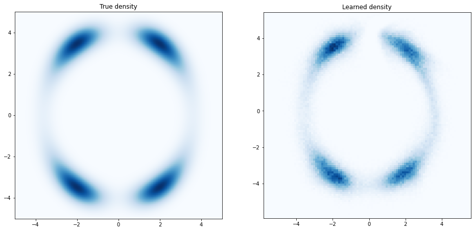

Figure 2.7: Learned density

2.6 More complex flows

2.7 Other versions

[TODO] Table from Papamakorios

3.1 Introduction

Up to now, the normalising flows were defined as a discrete series of transformations. If we go back to the reversible formulation of the flows, the internal state of the flow evolve as

\[\vec{x}_{i+1} = f(\vec{x}_{i}) = \vec{x}_{i} + \phi(\vec{x}_{i})\]

or

\[\vec{x}_{i+1} - \vec{x}_{i} = \phi_i(\vec{x}_{i})\]

This can be read as the Euler discretisation of the following ordinary differential equation:

\[\frac{d\vec{x}(t)}{dt} = \phi\left( \vec{x}(t), \theta \right)\]

In other words, as the steps between layers becoming infinitesimal, the flows become continuous, where \(\theta\) represent the layer’s parameters. Note that the parameters do not depend on the depth \(t\). As remarked by (Massaroli et al. 2020), this formulation with a constant \(\theta\) (instead of a depth-dependent \(\theta(t)\)) is the deep limit of a residual network with constant layer. We could be more general by using depth-dependent \(\theta(t)\) to create truly continuous neural networks.

Since \(\phi(\cdot)\) only depends on \(t\), we can define \(\vec{x}(t_1) = \phi^{t_1 - t_0}(\vec{x}(t_0)) = \vec{x}(t_0) + \int_{t_0}^{t_1}{\phi(\vec{x}(t))dt}\) and see that \(\phi^{t} \circ \phi^{s} = \phi^{t+s}\). Assuming, without loss of generality that \(t \in \left[ 0, 1 \right]\), \(\phi^1\) is a smooth flow called a time one map. Note that under the assumptions that \(\phi^t(\cdot)\) is continuous in \(t\) and Lipschitz-continuous in \(\vec{x}\), the solution is unique (Picard–Lindelöf-Cauchy–Lipschitz theorem).

This presentation of continuous flows is what (Chen et al. 2019) named Neural Ordinary Differential Equation.

Surprisingly, the log probability density becomes simpler in this continuous setting. The discrete formulation:

\[\log(P_Y(\vec{y})) = \log(P_X(\vec{x})) - \log(\left| \det\nabla \left( \mathbb{I} + \phi(\vec{x}) \right) \right|)\]

becomes

\[\frac{\partial \log(P(\vec{x}(t)))}{\partial t}=-Tr \left( \frac{\partial \phi(\vec{x}(t))}{\partial \vec{x}(t)} \frac{\partial \vec{x}(t)}{\partial t} \right)\] (See Appendix A of the paper for details.)

3.2 Continuous flows means no-crossover

Previously, in the context of discrete transformations, the transformation matrix (the Jacobian) could have strictly positive or strictly negative eigenvalues. This is not the case in a continuous context.

Let’s consider at a simple case in one dimension where we are simply trying to change the sign of a distribution.

For any value of \(t\), a transformation is only a function of the distribution density at that depth. The transformation does not depend on the trajectories reaching that depth. Therefore at the point of crossing, a transformation would not be able to create crossing trajectories.

Another way to look at this is to realise that at (or infinitesimally around) the point of crossing, the Jacobian of the transformation must have a negative eigenvalue to flip the volume. Starting from strictly positive eigenvalues, given that \(\phi(\cdot)\) is sufficiently smooth, reaching a negative eigenvalue implies going through 0, at which point the transformation ceases to be a diffeomorphim. This is contrary to the design of normalising flows.

Let’s look at what Torchdyn would produce. The dataset contains pairs of (-1, 1) and (1, -1).

n_points = 100

# The inputs
X = torch.linspace(-1, 1, n_points).reshape(-1,1)

# The reflected values
y = -X

X_train = torch.Tensor(X).to(device)
y_train = torch.Tensor(y).to(device)

# We train in a single batch
train = data.TensorDataset(X_train, y_train)
trainloader = data.DataLoader(train, batch_size=len(X), shuffle=False)

We define a LightningModule:

class LearnerReflect(pl.LightningModule):
    def __init__(self, model:nn.Module, settings:dict={}):
        super().__init__()
        self.model = model
    
    def forward(self, x):
        return self.model(x)
    
    def training_step(self, batch, batch_idx):
        x, y = batch      
        y_hat = self.model(x)   
        loss = nn.MSELoss()(y_hat, y)
        logs = {'train_loss': loss}
        return {'loss': loss, 'log': logs}   
    
    def configure_optimizers(self):
        return torch.optim.Adam(self.model.parameters(), lr=0.01)

    def train_dataloader(self):
        return trainloader

The ODE is a single perceptron:

# vanilla depth-invariant
f = nn.Sequential(
  nn.Linear(1, 64),
  nn.Tanh(),
  nn.Linear(64,1)
  )

# define the model
model = NeuralDE(f, solver='dopri5').to(device)

# train the neural ODE
learn = LearnerReflect(model)
trainer = pl.Trainer(min_epochs=100, max_epochs=200)
trainer.fit(learn)

# Trace the trajectories
s_span = torch.linspace(0, 1, 100)
reflection_trajectory = model.trajectory(X_train, s_span).cpu().detach()

plt.figure(figsize=(12,4))
plot_settings = {
  'n_grid':30, 
  'x_span': [-1, 1], 
  'device': device}

# Plot the learned flows
plot_traj_vf_1D(model, 
                s_span, reflection_trajectory, 
                n_grid=30, 
                x_span=[-1,1], 
                device=device);

# evaluate vector field
plot_n_pts = 50
x = torch.linspace(reflection_trajectory[:,:, 0].min(), 
                   reflection_trajectory[:,:, 0].max(), 
                   plot_n_pts)
y = torch.linspace(reflection_trajectory[:,:, 1].min(), 
                   reflection_trajectory[:,:, 1].max(), 
                   plot_n_pts)
X, Y = torch.meshgrid(x, y) 

z = torch.cat([X.reshape(-1,1), Y.reshape(-1,1)], 1)

# Field vectors
model_f = model.defunc(0,z.to(device)).cpu().detach()

fx = model_f[:, 0].reshape(plot_n_pts , plot_n_pts)
fx = model_f[:, 1].reshape(plot_n_pts , plot_n_pts)

# plot vector field and its intensity
fig = plt.figure(figsize=(4, 4))
ax = fig.add_subplot(111)

# Draws vector field itself
ax.streamplot(X.numpy().T, Y.numpy().T, 
              fx.numpy().T, fy.numpy().T, 
              color='black')

# Contour plot of the field's intensity 
ax.contourf(X.T, Y.T, 
            torch.sqrt(fx.T**2 + fy.T**2), 
            cmap='RdYlBu')

This simple example shows that in this form, Neural ODEs are not general enough.

3.3 Training / Solving the ODE

When optimising the parameters of discrete layers, we use backpropagation. What is the equivalent in a continuous setting?

Backpropagation works in a discrete context by propagate backward training losses which are allocated to parameters in proportion to their contribution to the loss and adjusting the parameters accordingly. The equivalent in a continuous context is the adjoint sensitivity method which originates from optimal control theory (see (Errico 1997) for example).

Given a loss defined as:

\[ \mathcal{L(\vec{x}(t_1))} = \mathcal{L} \left( \vec{x}(t_0) + \int_{t_0}^{t_1} \phi(\vec{x}(t), t, \theta) dt \right) \]

the adjoint \(a(\cdot)\) is defined as the gradient of the loss for a given hidden state evaluated at \(\vec{x} = \vec{x}(t)\):

\[ a(t) = \frac{\partial \mathcal{L}}{\partial \vec{x}(t)} = \frac{\partial \mathcal{L}}{\partial \vec{x}} \frac{\partial \vec{x}(t)}{\partial t} \]

The following figure explains what \(a(\cdot)\) represents: as \(t\) changes, so does the transformation \(\vec{x}(t)\) of the input (if looking from \(\vec{x}(t_0)\)). At a given step \(t\), the loss \(\mathcal{L}(\vec{x}(t))\) is a function only of that given state. The adjoint expresses (1) the changes of that loss and (2) expresses it as a function of the progress through the flow \(t\) instead of the value of the hidden state.

Figure 3.1: Backpropagation in time of the adjoint sensitivity (Source: (Chen et al. 2019))

A first order of approximation gives the following ODE (see (Chen et al. 2019) Appendix B.1. for details):

\[ - \frac{da(t)}{dt} = {a(t)}^\intercal \frac{\partial \phi(\vec{x}(t), t, \theta}{\partial \vec{x}(t)} \]

We write the negative sign in front of the derivative to make it more apparent that the adjoint sensitivity method is interested in tracking the backward changes of the loss: a positive derivative as \(t\) increases becomes a negative derivative as \(t\) decreases.

Deep learning libraries such a Pytorch, TensorFlow in Python, or Zygote.jl/Flux.jl/DiffEqFlux.jl in Julia provide automatic differentiation and a collection of bijections (to express the diffeomorphisms and loss function). They provide the infrastructure to express \(a(\cdot)\) and its derivative, track its changes and optimise the parametrisation \(\theta\) of the transformations. R has bindings to the Python libraries.

3.4 What parameters to optimise?

Recall that, unlike the initial introduction of the Neural ODEs, the general case has depth-dependent parameters \(\theta(t)\). There is no practical general implementation of those continuous networks. (Massaroli et al. 2020) describes two different approaches: hyper-networks where the parameters are generated by a neural network (one of the inputs being the depth), and what the paper calls Gälerkin-style approach. This approach uses a weighted basis of functions (think polynomials of a Taylor expansion or sine/cosine of a Fourier transform) limited to a few terms.

3.5 Increase the complexity of a flow: Augmented flows

As mentioned above, the basic continuous flows are not able to express something as simple as a change of sign of a distribution. This can be addressed with augmented flows (see (Dupont, Doucet, and Teh 2019)). The idea is to increase the dimension of the input: simply put, it embeds the flow into a space of higher dimension.

(Dupont, Doucet, and Teh 2019) demonstrate that this augmentation is efficient enough to achieve any transformation.

CHECK Appendix B.3 of (Massaroli et al. 2020)

3.6 Decrease the complexity of a flow: Regularisation and stability

Despite its advantages, continuous flows suffer from potential instability: it does not take much for a dynamic systems to exhibit a chaotic behaviour. This is all the more possible since the latent space dimension is the same as the dataset’s. A larger number of dimensions means more possible flows within that space. Depth-dependent parameters \(\theta(t)\), instead of a constant \(\theta\), increases that risk (using a constant being a form of regularisation). (See (Zhang, Wang, and Liu 2014) for a comprehensive review of the stability of neural networks.) Greater stability can be achieved by penalising extreme or sudden flow divergences where small changes in inputs yield large changes in output.

To quantify the propensity for chaotic behaviour, the literature is focused on the Lyapunov exponents (LEs) of the flows. What does LEs represent? Intuitively, you can imagine a point in space surrounded by a small volume \(V_1\). When that volume is carried by the flow (with time changing from \(t_1\) to \(t_2\)), it contracts and/or dilates to \(V_2\). LEs is a measure of this change \(V_2 / V_1\) expressed as a logarithm: if the volume is unchanged, the LE \(\lambda\) is 0 (\(e^\lambda = e^0 = 1\)). A contraction (resp. dilatation) has a negative (resp. positive) exponent. This is formulation has two benefits:

• An exponent can be of any sign, but the change of volume is always positive (a negative volume makes no sense); and,

• for time changing from \(t_1\) to \(t_2\), the exponent \(\lambda\) is consistently expressed as an instantaneous change independent of time: \(V_2/V_1 = e^{\lambda (t_2 - t_1)}\).

Adding a penalty term to the cost function are a natural solution:

• (Yan et al. 2020) proposes using an estimate of the Lyapunov exponent. However, their proposal is to make this estimation along the flows; in essence, they regularise each flow (from an infinitesimal volume to another along segments of that flow) to avoid successive cycles of contraction/dilatation. Intuitively, this favours flows in the form of funnels (contraction) or horns (dilatation). It is however computationally expensive.

• (Massaroli et al. 2020) proposes to only calculate between \(t=0\) and \(t=1\) (with \(\mathcal{L}_{reg} = \sum\limits_{i}^N \left|| \phi^1(t, x(1), \theta(1)) \right||_2\) for a training batch of size \(N\)). If \(\phi^1\) is zero, there is no change between the initial and final volume of a flow line.

3.7 Other

Previously mentioned generative models can be improved with normalising flows

Flow-GAN Grover, Dhan Ermon, Flow-GAN combining max Likelihood and adversarial learning and generative model