DRAFT 1

We all have laptops. But le’ts face it, even in times of 32GB of RAM and NVMe2 drives, forget about running any interesting TensorFlow model. You need to get an external GPU, build your own rig, or very quickly pay a small fortune for cloud instances.

Back in 1993, I read a paper about growing neural networks neuron-by-neuron. I have no other precise recollection about this paper apart from the models considered being of the order of 10s of neurons and the weight optimisation being made on a global basis, i.e. not layer-by-layer like backpropagation. Nowadays, it is still too often the case that finding a network structure that solves a particular problem is a random walk: how many layers, with how many neurons, with which activation functions? Regularisation methods? Drop-out rate? Training batch size? The list goes on.

This got me thinking about how a training heuristic could incrementally modify a network structure given a particular training set and, apart maybe from a few hyperparameters, do that with no external intervention. At regular training intervals, a layer¹ will be modified depending on what it seems able or not to achieve. As we will see, we will use unsupervised learning methods to do this: a layer modification will be independent of the actual learning problem and automatic.

Many others have looked into that. But what I found regarding self-organising networks is pre-2000, and nothing in the context of deep learning. So it seems that the topic has gone out of fashion because of the current amounts of computing power, or has been set aside for reasons unknown. (See references at the end). In any event, it is interesting enough a question to research it.

Background

Let us look at a simple 1-D layer and decompose what it exactly does. Basically a layer does:

\[ \text{ouput} = f(M \times \text{input}) \]

If the input \(I\) has size \(n_I\), the output \(O\) has size \(n_I\), and \(f\) being the activation function, we have (where \(\odot\) represents the matrix element-wise application of a function):

\[ O = f \odot (M \times I) \]

Then, looking at \(M\), what does it really do? At one extreme, if \(M\) was the identity matrix, it would essentially be useless (bar the activation function²). This would be a layer candidate for deletion. The question is then:

Looking at the matrix representing a layer, can we identify which parts are (1) useless, (2) useful and complex enough, or (3) useful but too simplistic?.

Here, complex enough or simplistic is basically a synonym of “one layer is enough”, or “more layers are necessary”.

The idea to look for important/complex information which where the network needs to grow more complex; and identify trivial information which can be discarded, or can be viewed as minor adjustments to improve error rates (basically overfitting…)

Caveat: Note that we ignore the activation function. They are key to introduce non-linearity. Without it, a network is only a linear function, i.e. no interest. They have a clear impact on the performance of a network.

Singular matrix decomposition

There exists many ways to decompose a matrix. Singular matrix decomposition (SVD) \(M = O \Sigma I^\intercal\) is an easy and efficient way to interpret what a given matrix does. SVD builds on the eigenvectors (expressed in an orthonormal basis), and eigenvalues. (Note that \(M\) is real-valued, so we use the transpose notation \(M^\intercal\) instead of the conjugate transpose \(M^*\).)

In a statistical world, SVD (with eigenvalues ordered by decreasing value) is how to do principal component analysis(PCA).

In a geometrical context, SVD:

• takes a vector (expressed in the orthonormal basis);
• re-expresses onto a new basis made of the eigenvectors (that would only exceptionally be orthonormal);
• dilates/compresses those components by the relevant eigenvalues;
• and returns this resulting vector expressed back onto the orthonormal basis.

As presented here, this explanation requires a bit more intellectual gymnastic when the matrix is not square (i.e. when the input and output layers have different dimensions), but the principle remains identical.

Where next?

Taking the statistical and geometrical points of view together, the layer (matrix \(M\)) shuffles the input vector in its original space space where some specific directions are more important than others. Those directions are linear combinations of the input neurons, each combinations is along the eigenvectors. Those combinations are given more or less importance as expressed by the eigenvalues. (Note that the squares of the eigenvalues expressed how much information each combination brings to the table.)

Intuitively, the simplest and most useless \(M\) would be the identity matrix (the input units are repeated), or zero matrix (the input units are dropped because useless). Let us repeat the caveat that the activation function is ignored.

If compared to the identity matrix, the SVD shows that \(M\) includes (at least) two types of important information identified:

• What are interesting combinations of the input units? This is expressed by how much the input vector is rotated in space.
• Independently from whether a combination is complicated or not (i.e. multiple units, or unit passthrough), how an input is amplified (as expressed by the eigenvalues).

The idea is then produce a 2x2 decision matrix with high/low rotation mess and high/low eigenvalues.

A picture is gives the intuition of what we are after:

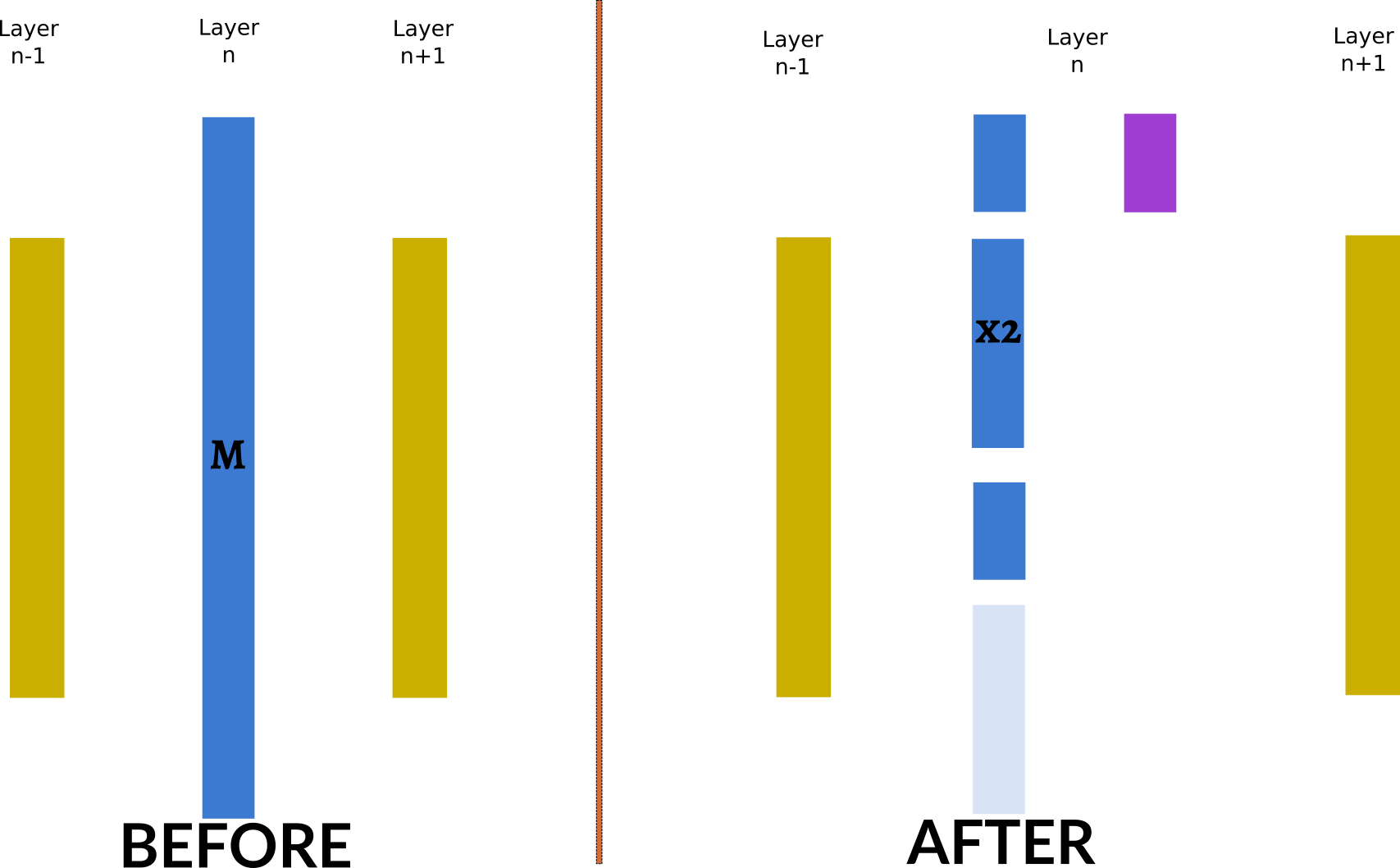
Transformation of the Layer Matrix

Looking from top to bottom at what the “after” matrices would be:

• Part of the original layer, immediately followed by a new one (we will see below what that would look like). The intuition is that this layer is really messing things up down the line, or seems very sensitive.

• Part of the original layer where the number of units would be increased (here doubled as an example).

• Part of the original layer kept functionally essentially as is.

• Delete the rest which is either not sensitive to input or outputs nothings. This would be within a certain precision. That is basically a form of regularisation preventing the overall model to be too sensitive. I am aware that there are other types of regularisations, but that will go in the limitations category.

The next layer would take as input all the transformed outputs.

In practice, the picture presents the matrices separated. This is for ease of understanding. In reality the same effect would be achieved if the three dark blue sub-layers are merged in a single layer.

Back to SVD

Let us assume that there are \(n\) input units and \(m\) output units. \(M\) then is of dimensions \(m \times n\). The matrices of the SVD have dimensions:

\[ \begin{matrix} M & = & O & \Sigma & I^\intercal \\ m \times n & & m \times m & m \times n & n \times n \\ \end{matrix} \]

Note that instead of using \(U\) and \(V\) to name the sub-matrices of the SVD, we use \(I\) and \(O\) to represent input and output.

The \(I\) and \(O\) can be written as:

\[ I = \begin{pmatrix} | & & | \\ i_1 & \cdots & i_m \\ | & & | \\ \end{pmatrix} \qquad \text{and} \qquad O = \begin{pmatrix} | & & | \\ o_1 & \cdots & o_n \\ | & & | \\ \end{pmatrix} \]

Then:

\[ \begin{aligned} M & = O \Sigma I^\intercal \\ & = \begin{pmatrix} | & & | \\ o_1 & \dots & o_m \\ | & & | \\ \end{pmatrix} \times \\ & \times \begin{pmatrix} \sigma_1 \\ & \sigma_2 \\ && \ddots \\ &&& \sigma_r \\ &&&& 0 \\ &&&&& \ddots \\ &&&&&& 0 \\ \end{pmatrix} \times \\ & \times \begin{pmatrix} - & i_1 & - \\ & \vdots & \\ - & i_n & - \\ \end{pmatrix} \end{aligned} \]

where \(\Sigma\) has \(r\) non-zero eigenvalues.

Regularisation

At this stage, we can regularise all components.

[TODO] Other Principal Components methods

SVD is PCA. Projects information on hyperplanes.

Reflect on non-linear versions: Principal Curves, Kernel Principal Components, Sparse Principal Components, Independent Component Analysis. (_Elements of Statistical Learning s. 14.5 seq.).

Limitations and further questions

Litterature

Here are a few summary litterature references related to the topic.